Data Analysis and Presentation Skills Part 5 potx
Bạn đang xem bản rút gọn của tài liệu. Xem và tải ngay bản đầy đủ của tài liệu tại đây (597.12 KB, 19 trang )
Diet B and Diet C as these are the labels on the worksheet. Sometimes we may
want to change these or correct mistakes. Enter edit mode by selecting the
graph and choose Source Data after clicking with th e right mouse button. T his
takes you back to the step where you selected rows instead of columns. Click on
the Series tab. From here you are able to select th e data in each row and in the
name box rename each label in the legend, as shown in Figure 3.26.
A further option that we might want to include is to show a table containing
the data itself beneath the plot. Once the char t is complete you can edit the
graph (by clicking on it) and th en select C hart Options from the menu. Click
on the Data Table tab and by selecting Show Data Table, as can be seen in
Figure 3.27, a data table i s displayed beneath the plot.
Grouped 3-D ba r charts
T he information can be conveyed again slightly d i¡erently by using a three-
dimensional bar chart. Here bars may be placed in front of or behind each
other and so give emphasis to components of the plo t.
In Excel, re-plot the weight loss information; this time select the 3-D
Column option, placing the data back into columns instead of rows. On the
three -dimensional plot it would be more appropriate to have the label ‘weight
loss’at the top of the ax is with the text written horizontally (remember we read
from left to right) rather th an written vertically so that the reader needs to turn
through 908 to be able to read it. To adjust the position of the label, select the
64 3 PRESENTING SCIENTIFIC DATA
Figure 3.25 Stacked column chart
65PRESENTING GRAPHS AND CHARTS
Figure 3.26 Editing the legend
Figure 3.27 Displaying data beneath a graph
label to enter edit mode and right click the mouse button. From the options
choose Format Axis Title. You are then confronted with options to alter the
text alignment of the label. Use th e mouse button to alter the orientation of the
text as shown in Figu re 3.2 8 an d con¢rm you r choice. You should then have a
plot that looks very similar to that shown in Figure 3.29.
Finally, exp erim ent with these data by changing the ove rlap of the bars in
the chart. If we look at the plot we can see that the data for the male subjects
‘overshadows’ that for the females. Thi s is because the weight loss was greater
66 3 PRESENTING SCIENTIFIC DATA
Figure 3.28 Aligning text in titles
Figure 3.29 Three-dimensional plots
for the male subjects. It would be preferable for the female data to appear at the
front of the chart, so how do we accompl ish this? By clicki ng on the plot, enter
edit mode. Select the bars representing the male subjects and click on th e right
mouse button. Choose Format Data Series fro m the menu and then select the
Series Order tab. Using the move up and move down buttons you are able to
alter th e position of the bars on the graph as shown in Figure 3. 30.The data are
more aptly presented with the female data columns being in front of those for
the males, so select this option and return to the worksheet. Although the
display is improved, to provide further contrast between the male and female
data it would be better if the bars at the front of the graph were lighte r than
those behi nd. Using the editing options th at you applied in section 3.1, change
the bar colours until you have a plot similar to that shown in Figure 3.31.
Printing bar and column graphs
The graphs shown on you r computer monitor are usually impressive as some
good comparisons are shown using appropriately contrasting colours.When it
comes to printing, however, some of the contrasts may be lost, partic ularly
wh ere very light colours have been used against an equally light background.
For bar, column and pi e charts it may be necessary to select patterns. Here are
67PRESENTING GRAPHS AND CHARTS
Figure 3.30 Changing the s eries order in graphs
a few tips on how to make the patterns on your plots look equally as good
when printed in black and whi te:
. Use d ots and lines as ¢ller patterns as these give good results. Lines are
better if they are slanted rather than horizontal or verti cal. Avoid some of
the graduated shading that is available in Excel as this may cause problems
in contrasting with the background shades.
. Avoid using patterns that are too busy.These detract from the plot.
. Colum ns that are comple tely black should be avoided as these may smudge
on prin ting and may also dominate the chart. They also use up vast
quantities of ink or toner if you are producing full-page plots.
. White may be used for emphasis and does not have the e¡ect of being too
overpowering. It is particularly e¡ective if you are tryi ng to emphasize a
‘control’ or ‘no response’ g roup.
. Avoid using too many di¡erent patterns on a chart as the result is
confusing. Do not place patterns that are similar too close together
otherwise the contrast is lo st.
Pie charts
T hese are the main alternative to bar charts and are useful i n making
comparisons of proportions. Using a pie chart it is di⁄cult to read individual
68 3 PRESENTING SCIENTIFIC DATA
Figure 3.31 Completed graph showing emphasis by changing colours and patterns
values, particularly where there are several categories, so the pie chart tends to
be used for the purpose of providing an ove rview. By using the feature in E xcel
to remove a ‘slice’of the pie, a particular aspect of the data can be emphasized.
Taking the data from E xerc ise 3.3 (Table 3.3 ) we will s ee how to construct a
pie ch art to represent the decrease in body weight for the male subjects. Using
the data on your worksheet, select the data for the male subjects and click on
the Chart Wizard button. From the list of available options select Pie with a 3-
D visual e¡ect. Continue through the chart optio ns to complete the plot which
should be similar to that in Figure 3.32. Although the three-dimensional pie is
e¡ective it would be easier to judge the di¡erent proportions if the position of
the pie was adjusted. This is accomplished in Excel by selec ting the pie; to
69PRESENTING GRAPHS AND CHARTS
Figure 3.32 Pie chart
Figure 3.33 Changing the angle of the ¢rst slice
accomplish this click on it, but in doing so make sure that handles appear on
every slice of th e pie. Finding exactly the right selection can sometimes be
di⁄cult; editing wi th di¡erent selecti ons can pull apart slices or expand the
top or sides of the pie. You will need to experiment with these features to ¢nd
out exactly how they work. Once you have successfully selected the pie pieces,
however, you should then be able to s elect the option to Format Data Series.
From this go to the Options menu. Here you are able to move the angle of the
¢rst slice. By increasing the angle you will cause the pie to rotate, as shown in
Figure 3.33.Try this option until you reach the p oint where you feel that the pie
pieces are now much easier to compare than in th e original plot, and then
con¢rm your choice.The plot shows that the least weight loss was experienced
with Diet A. To place emphasis on this point we could remove or ‘explode’ a
piece of pie. By clicking on the slice of pie for Diet A it should b e possible to
select and then drag the slice from the other pieces. Try this for yourself. The
¢n ished plo t should b e comparable to that shown in Figu re 3. 34.
Line graphs
Line graphs are use d to compare t wo variables and show the relationship that
exi sts between them. Usual ly the independent variable is plotted on the x-axis
and the variable that is depende nt on x on the y-axis. An independent variable
is one that is controlled by the experimenter, so this will include variables such
as time, tempe rature, pH, etc. The dependent variable is dependent on the
value of x and so will change with x. Line graphs show an ordered relationship
between sets of data so that if the value o f one variable is known the graph may
be use d to predic t the value of the o ther.
70 3 PRESENTING SCIENTIFIC DATA
Figure 3.34 Pie chart with slice removed
We will use as an example a kinetics plot where the concentration of a drug
is seen to change with time. In the example in Table 3.4 there are two drug
concentrations that are being investigated so we can use a multi-line graph.
Exercise 3.4
Enter the data from Table 3.4 on your worksheet. Using the
option for XY (Scatter) and Data points connected by smooth
lines, plot a multi-line graph for both drugs on the same plot. In
producing the labels for this plot you will need to insert the
units for concentration. These are mg·ml
71
. To insert symbols
into Excel that will appear on worksheets and in graphs and
charts you can use the symbol codes (listed in the Appendix).
To insert a symbol press the Alt key on the computer, then
enter the numerical code using the Number pad on the right-
hand side of the keyboard. On releasing the Alt key, the symbol
will appear on your worksheet. Complete the plot by adding
titles and labels. You should now be familiar with inserting error
bars, so include the standard deviation on your plot, placing +
error bars on the upper line and 7 error bars on the lower line.
Your graph should appear as in Figure 3.35.
We will now see how we can transform the data by using a
semi-logarithm ic plot. These plots are often used with kinetic
data where the y-axis is represented logarithmically. Click on
the chart to enter edit mode and select Chart Type from the edit
menu (produced by right clicking the mous e button). Click on
71PRESENTING GRAPHS AND CHARTS
Table 3.4 Concentrations of drugs A an d B against time
Time (h)
Concn drug A
(mg/ml)
Concn drug B
(mg/ml) SD (A) SD (B)
1 100.1 120.2 5.6 6.6
2 50.2 100.3 2.1 5.4
3 25.5 80.4 1.9 4.3
4 20.2 62.5 1.4 3.6
5 15.6 51.4 1.1 2.0
6 12.1 39.6 0.8 1.5
710.333.50.50.9
72 3 PRESENTING SCIENTIFIC DATA
Figure 3.35 Line graphs
Figure 3.36 Selecting a logarithmic line graph from chart options
the Custom tab. Here you will find a number of graphs that do
not appear under the standard options. Selec t Logarithmic
from the list. A preview of the graph appears on which the y-
axis is a logarithmic scale as seen in Figure 3.36. Confirm your
choice and complete the graph.
Combination plots
Sometimes we may want to demonstrate a change in two variables, each with
di¡erent units of measurement, on the same graph. This is where we need to
use what is known as a combination plot. This plot has two y-axes ; di ¡erent
units and scales can be used on each axis and the data are presented as a
combination of a bar chart and line plot.
Exercise 3.5
The data in Table 3.5 compares the change in heart rate and
diastolic blood pressure in a hypertensive patient during a
period of moderate exercise on a treadmill. As we are
interested in how ea ch variable chang es with time a com bina-
tion plot would be ideal to show how the two variables might be
related.
Enter the data from Table 3.5 on your worksheet and using
Chart Wizard, choose one of the combination chart options.
This will again be found on the Custom Types selection under
73PRESENTING GRAPHS AND CHARTS
Table 3.5 Mean diastolic blood pressure in a hypertensive patient during moderate exercise
Time (minutes) Diastolic BP (mmHg) Heart rate (bpm)
10 80 80
20 85 85
30 93 90
40 98 100
50 9 9 110
60 105 120
Line-Column on 2 axes (we select two axes rather than one as
the units for blood pressure and heart rate are different). The
preview for the chart will show that all three variables – time,
blood pressure and heart rate – are plotted on the graph.
Clearly this is wrong as the x-axis should be time (as this is the
independent variable) and not the arbitrary numbers inserted
by Excel. To amend the plot select the Series tab and click on
Time from the Series list and then Remove. The time data now
need to be re-inserted under category x-axis labels (as shown
in Figure 3.37), so click in this box and insert the cell references
for time, but excluding the label Time from your selection. The
preview shows the graph correctly plotted and we can complete
the graph by adding titles and then make our comparison of the
change in heart rate and blood pressure in the patient over
time.
74 3 PRESENTING SCIENTIFIC DATA
Figure 3.37 Semi-logarithmic options for line plots
WEB SUPPORT – SECTION 3
Here you will ¢nd plenty of data with which to experime nt with di¡erent
types of plots.You will be able to compare the ¢ni shed result with ready-
prepared charts so that you can see whether you have presented the data
correctly. You’ll also ¢nd more hints and tips on data presentation, plus
any information about Excel up dates that a ¡ect plotting functions.
75PRESENT ING GRAPHS AND CHARTS
4
Preliminary Data Analysis
Having reviewed data from investigations by plotting graphs,
we may conduct some preliminary statistics before moving
on to testing the data. Usually we are interested in looking
for trends in data, determining the variability of results and
considering its validity as a representative sample from the
population from which it was drawn. This section reviews
some of the techniques used for preliminary data analysis.
4.1 Descriptive statistics
As the name suggests, these are statistics that we calculate in order to
summari ze the data from our stu di e s.They are used to give a description of the
data by determining measures of locatio n and to express i ts variability. Each of
these aspects will be discussed in turn.
Measures of location
There are three main types of measures of location, these are known as the
(arithmetic) mean, also known as the average, the median and the mode. Each
has d i¡e ren t prope rties and use s.
Data Analysis and Presentation Skills by Jackie Willis.
& 2004 John Wiley & Sons, Ltd ISBN 0470852739 (cased) ISBN 0470852747 (paperback)
The mode
T he mode is the category or class of variable with the mo st observations in it,
i.e. the most fre quently occu rring value.Table 4.1 shows the number of hours a
sample of students spent watching the television each week. As we can see
from the table, the mode is 10.5 hours as this is the most frequently occurring
time. Sometimes there may be two values for the mode, in which case the
sample is said to be bimodal. The mode does not indicate the centre of the
sample, only those values that occur the most often.
The mode is very easily calculated in Excel. Enter the raw data from the
worksheet (the raw data is the individual value s for each of the stude nts and so
will exclude the summary statistics that have been calculated). Choose a cell on
the worksheet in which you would like the modal value placed, then cl ick on
the Pas te Function (see Section 3.1) and select MODE from the Statistical
menu. You will be prompted to enter th e cell references for the cells that
contai n the raw data, con¢ rm your s elec tion and the value for the mode should
appear in the cell that you selected on the worksheet.
The median
If all of the observations in a set were placed in ascending order, then the
median would be the middle observation. The median will have as many
observations above it as below it. If we look again at Table 4.1, but this time
sort the values in ascending order, we can see that 10.5 hours is the middle
value as th ere are exactly four values above and four values b elow this number.
T he median therefore gives us an indicat ion of the value in the central location
of the sample, but it does not summarize all of the data. The med ian provides
the middle value of the distribution.Where there is an even number of values,
the median wil l be the average of the two middle values (e.g. if there were eight
in our sample and the two middle values were 10 and 10.5, then the me dian
would be 10.25 hours).
The median can be calculated from Excel in the same way as the mode.
Using the data entered on the worksh eet, click on the Paste Function and select
78 4PRELIMINARYDATAANALYSIS
Table 4.1 Number of hours per week spent watching telev ision by a group of students
Mean Mode Median SD
12 13.5 10 10.5 7 10.5 12 9.5 10.5 10.6 10.5 10.5 1.8
Mean Mo de Median SD
7 9.5 10 10.5 10.5 10.5 12 12 13.5 10.6 10.5 10.5 1.8
MEDIAN from the list of S tatistical f unctions. After entering the cell refer-
ences the value for the median will appear on the worksheet.
The mean (average)
In contrast to the median, the mean summarizes all of the data and is
calculated by a ddin g all of the values and dividing th e sum by the
number of observations. So from the data in Table 4.1 the mean value would be
95.5/9 ¼10.6 hours. Although the mean provide s a value that includes all of
the data, one problem is its sensitivity to any extreme values that may occur
within a data set. If we had an additional student in the sample that watched
television for 40 hours per week, th e mean value would beco me (95.5 + 40)/10,
i.e. 135.5/10 ¼13.6 hours. Clearly the value of the mean is no longer a good
measure of the centre of the sample. If we compare this with the me dian value,
the additional obs ervation does not alter it in any way as the median value is
still 10.5 hours.
We have already used Excel to calculate the mean as this was used in
Section 3 with the butter£y data.The mean is denote d as the AVERAGE in the
Statistical fu nctions in Excel.
Choosing bet ween using the median or the mean
When deciding which measure to use, the shape of the distribution from
which the sample is taken becomes the deciding factor.Where a distribution is
symmetrical, showing a normal (bell-shaped) pattern as can be seen later in
this section i n Figure 4.4, the mean value is preferre d as it uses all of the
observations in its calculation. Where a distribution is skewed, therefore
containin g an excess of extremely large or extremely small observations, the
median is preferred as it is insensitive to thes e extremes. If the mean were to be
used, a shift in its value wou ld have occurred either to the left or to the right of
the distribution, depend in g on whether is it positively or negatively skewed,
and therefore the mean value would be clearly i nappropriate. These aspects of
distributions are fur ther discussed in section 4.2.
Measures of variation
The measures of variation of a set of observations are described by the ran ge,
variance and standard deviation. Each of these is used to determine the
variability within a set of data. If we return to the data in Table 4.1 and include
79DESCRIPTIVE STATISTICS
data from an extension of the original investigation. All of the students in the
original study lived in halls of residence; we will assign them as Group 2. A
fur ther g roup of nin e stu dents was investi gate d , all of whom live d at home.
T he number of hours per we ek spent watching television was compared
between the two groups.The data are shown in Table 4.2.
Simply by looking at the information in th e table we can see that there is a
di¡erence between the two groups.The mean number of hours spent watching
the television is exactly the same for each group, but there is clearly more
variability in the number of hours in Group 1 than in Group 2, and values for
the median and mode are di¡erent. There needs to be some means of
representing the variability between the groups.
The range
T he range is a very basic means of expressing the extent of variation in a
sample; it is simply the d i¡erence between the maximum and minimum values.
So for Group 1 this will be:
2077. 5 ¼12 .5 hours
and for Group 2 this will be:
13.577 ¼6. 5 hours
Like the median and mode, the range only uses a small part of the data (largest
and smallest values) and so does not re£ect the true variation between all of
the values.
The standard deviation and variance
T he standard d eviation and variance indicate how closely packed arou nd the
mean the values in a variable are. The standard deviation and variance use all
the information in the sample and have a number of mathematical properties
which enable them to be used in various statistical tests.
80 4PRELIMINARYDATAANALYSIS
Table 4.2 Number of hours per week spent watching television by two groups of students
Mean Mode Median SD
Group 1 9 10 9.5 8.5 11 9 10.5 7.5 20 10.6 9 9.5 3.7
Group 2 12 13.5 10 10.5 7 10.5 12 9.5 10.5 10.6 10.5 10.5 1.8
Va r ia n c e :
variance ¼
P
ðx ÀmeanÞ
2
n À1
ðEquation 4:1Þ
where x is each individual observation in the sample.
T he variance i s calculated by subtracting th e mean from each individual
value in the sample and taking the total of the sums of the squares of th e
deviations from the m ean values.The resulting value for the variance is usually
a large number in relation to the mean value. The measure of variation is
therefore taken to be the standard deviation which is the square root of the
variance.
Standard deviation:
SD ¼
p
ðvarianceÞðEquation 4:2Þ
From looking at these equations it is easy to see how the variance and SD are
able to represent the variab ility in the data in comparis on to its mean value.
The more variation there is in a sample, the greater the deviations of the value s
from the mean. As the standard deviation and variance use all of these devia-
tions in their calculation, they truly re£ect the variability in the data. Looking
back at the data inTable 4.2 we can see how this helps us to interpret the results
for the two groups of students. The mean value may be the same, but there is
far more variability in the ¢rst group than in the second as the standard
deviations are 3.7 and 1.8 hours respectively. The variabil ity for Group 1 can be
mainly attributed to one very large value: one student watched television for 20
hours. This clearly has an e¡ect on the distribution of the results, as the other
students tended to have much lower viewing times. Thi s is con¢rmed by
comparing the values for the median, mode and range.
We have already seen how Excel can be used to calc ulate the standard deviation
of data, using the exam ples with the butter£ies in section 3.1. A far more useful
facility in Excel is to use the Descriptive Statistics function that will supply all
of the descriptive stati stics for a set of data and so save time in calculating each
parameter individually.
81DESCRIPTIVE STATISTICS
Descriptive statistics in Excel
Input the data in Table 4.2 into an Excel spreadsheet. From the Tools menu
select Data Analysis.
Note : If the Data Analysis option does no t appear at the bottom of the
Tools menu then you will need to load this function either from your
network or from the Microsoft O⁄ce CD. From the Tools drop down
menu, select Add-Ins and from the list provided check the box against
A nalysis ToolPak. After you have s elec ted OK, the ToolPak should be
loaded and you should then ¢nd Data Analysis under the Tools menu
when this is reselected.
Choose Descriptive Statistics from the list provided. A dialogue box should
then appear in which you input the range of cells for the data arran ged on the
worksheet. Include the labels in the selection and then check the box Lab els to
show that these are include d, as shown in Figure 4.1. If your data are in rows
rather than in columns then also ensure that you change the option in the
dialogue box. Check the Summary Statistics to indicate that you want these
displayed and then having chosen where on the worksheet the results should
appear (it is usually a good idea to choose a new workshee t where there is a lot
of data), click OK.
Your workb ook will be updated with a table of summary statistics as shown
in Figure 4.2 .
Standard error
One of the descriptive statistics produced by Excel is the standard error,
sometimes abbreviated as SEM (standard error of the mean). The re is no
function in the Paste Function to calculate this value by itself, so i t has to be
calculated by using a formula. The standard error is by de¢nition an estimate
of the standard deviation of the distribution of the mean, describing how
spread out th e distribution of the p opulation from which the sample was taken
actually is. The mean that is calculated from a sample is never the same as the
value for the mean if the data for the entire population were to be include d.
T he standard error provides an estimate of how closely the sample m ean
represents the tr ue mean for the p opulation. So when the standard error is low,
it is more likely that the sample mean is a good re£ect ion of the value for the
82 4PRELIMINARYDATAANALYSIS