Data Analysis and Presentation Skills Part 6 pps
Bạn đang xem bản rút gọn của tài liệu. Xem và tải ngay bản đầy đủ của tài liệu tại đây (689.37 KB, 19 trang )
true population mean. The equatio n for the standard error may be seen in
Equation 4.3:
SEM ¼
standard deviation
H number in sample
ðEquation 4:3Þ
If we wanted to check that the value of the standard e rror calculated in the
Descriptive Statistics function was correct then we would ins ert the following
formula into a cell on the spreadsheet, using the data from Group 1 as an
example:
¼3.7/SQRT(9)
83DESCRIPTIVE STATISTICS
Figure 4.1 Descriptive Statistics functions in Excel
where 3.7 is the standard deviati on of the sample , for which there were nin e
observations, so it could be calculated by:
¼STDEV (range of values in sample)/SQRT (number in sample)
When presenti ng graphs showing mean values it is usually expected that
error bars are included by using either the standard deviation values to
demonstrate the variability in the sample, or the standard error to demonstrate
the deviation of the sample from the true population mean.
Kurtosis and skewness
Values for ku rtosis and skewness are also produced by the Des criptive
Statistics function.These are used to characterize the data relative to a normal
distribution. Skewness is a measure of symmetry.Where data are symmetri cal
about the mean the skewness would be expected to have a value of around 0. If
data are skewed to the left or right the n the ce ntre of the data is not around the
mean and so a negative or positive value for skewness would be obtained.
Skewed distributio ns are further discussed in sectio n 4.2.
Kurtosis compares the shape of the data to a normal distribution and is a
measure of whether the data tend to b e peaked or £at .Where a hi gh value for
kurtosis is obse rved, data show a distinct peak about the mean and then
decl ine rapidly. For lower kurtosi s values, data are more spread out, giving a
£at top to the shape of the distribution rather than a peak. A value of around 3
would represent a normal distr ibution.
84 4PRELIMINARYDATAANALYSIS
Figure 4.2 Descriptive Statistics for the television viewing data
Coefficient of variation
This function also does not appear in Excel but is a very useful parameter to
calculate. The coe⁄cient of variation represents the standard deviation as a
percentage of the mean value; it is particularly useful when comparing the
reproducibility of results. In quantitative analytical methods, th e coe⁄cient of
variation is used as a measure of pre cision i n quality control determinations.
T he coe⁄cient of variation is calculated as shown in Equation 4.4:
coefficient of variation ¼
standard deviation
mean
 100% ðEquation 4:4Þ
The coe⁄cient of variation is usually given as a percentage and expresses the
variability (from the standard deviation) of the sample compared to the mean
valu e. It is a useful parame ter to use when comparing two or more samples
with di¡erent means to see if the variabili ty is the same in each sample.
Exercise 4.1
If we take as an example a laboratory analysis conducted by
two students. Each performed an assay to determine the
protein concentration of a sample containing 125 mgÁml
À1
of
protein. Each repeated the analysis 10 times and the results
are shown in Table 4.3.
Enter the data on a spr eadsheet in Excel and perform the
descriptive statistics on the data. Using the data for the mean
and standard deviation for each sample, enter the following
equation into one of cells on the worksheet, inserting the
appropriate value for the mean and standard deviation in each
case:
¼(value for standard deviation/value for the mean)
*
100
When comparing the means you should find that both students
have a mean value of 125 mgÁml
À1
from their protein determi-
nations, but student 2 has a more precise technique as the
coefficient of variation is 2.3 per cent for their analysis
compared with 7.3 per cent for student 1.
85DESCRIPTIVE STATISTICS
4.2 Frequency distributions
When we conduct scien ti¢c investigations, we collect data by taking samples
from much larger populations. In order to learn something about the popula-
tion we use de scriptive statistics, but we also need to examine the
characteristics of the dis tribution in order to determine the best way to
summarize and analyse data.
In Section 3 we learnt abou t pres enting data in the form of bar charts.We
can draw bar charts of data in which we me asure frequency (the number of
times a part icular occurrence takes place, for example the numb er of indivi-
duals in a population with blue eyes); if we draw a li ne at the midpoint of the
bar then we obtain a frequency polygon. Inc reasing the number of bars in the
plot, providing there is su⁄cient data to do so, will even tually produce a
smooth curve, the shape of which will tell us something about the character-
istics of the population. Figure 4.3 shows how a frequency polygon may be
produced from a bar chart, using data showing height of a sample of adults
from a population. This type of bar chart is known as a histogram.
86 4PRELIMINARYDATAANALYSIS
Table 4.3 Protein determinations performed by two students with a sample125 mgÁml
À1
Student1 125 120 122 130 115 140 130 121 125
Student 2 121 124 127 122 125 126 1 28 126 12 6
Figure 4.3 Normal distribution of heights of subjects
87FREQUENCY DISTRIBUTIONS
Figure 4.4 Skewed and bimodal distributions
Where the resulting frequency polygon re sembles a bell-shape we can
see that the population is symmetrical and the shape o f the curve is said to be
‘bell-shaped’. At e ach end, or tail, of the curve, there is a small nu mber of
extremely small or extremely large values, but the majority of the observations
fall in the middle part of the curve, i.e. they are centred around the value for
the mode. If we were to calculate the mean and the median for these data we
would ¢nd that values would be virtually identical. A curve is said to follow a
normal distribution where this occurs, so as the mean will re£ect the central
tendency of the distribution it should also resemble the midpoint of the
distribution, represented by the median.
It is useful when considering the shape of a population to look at the tail of
the curve that is produced. In Figure 4.4 we can see two distributions that
cannot be normal as they do not follow a bell-shape; these are known as
skewed distributions, of which there are two types, p ositive an d negative (see
also the subsection ‘Descriptive statistics in Excel’ in section 4.1).
A d istribution with a positive skew will contain more extremely large value s
than extremely small ones and therefore resembles Chart A. Clearly the mean
calculated for these data would not represent the central location of the
distribution. Similarly, if we consider Chart B there are clearly more extremely
small values than extremely large ones, in which case the data are n egatively
skewed. For each of these cu rves, the best measure of the central tendency for
the data would be represented by the median value and not the mean.
Sometimes the shape of this distribution appears as if two normal (bell-
shape d) distributions have been comb ined together, as shown in Chart C in
Figure 4.4. This would su ggest that there is a mixed population, which might
arise where a population contains two species.
In plotting these cur ves we have split the data into groups, or inte rvals, that
are equal ly spaced apart.The more intervals we are able to divid e the data into,
the more well-de¢ned the curve becomes.We will see how by using raw data
for heights of individuals we are able to produce a frequency dis tribution and
how the Excel Paste Function may be applied to aid this process.
Exercise 4.2
The data in Table 4.4 have been collected from a sample of 40
individuals from a population. Enter the data in one column in a
new workbook in Excel. The height of each subject was
recorded to the nearest centimetre, so in terms of the absolute
accuracy of the results, a person whose height is between
88 4PRELIMINARYDATAANALYSIS
153.5 and 154.4 cm would still be recorded as 154 cm (by
rounding up or down). Height would therefore be described as
being a continuous variable, but because we are taking
recorded measurements correct to the near est centimetre, we
are sampling discrete values.
The data on the worksheet make little sense as they stand
and need to be organized. The first, most obvious step is to
place them in order. Using the DatajjSort command (as
described in Section 3), organize the data into ascending
order. Look down the column of data to see the results. We
can now see that the smallest (minimum) value for height
is 147 cm whereas the la rgest (maximum) is 188 cm, so the
heights of the individuals range from 147 to 188 cm. Even
after sorting, the data are still difficult to interpret as each
value has to be examined in relation to all the others (and
what if we had thousands of measurements?). The next
stage is clearly to group the data; this is done by dividing it
into classes – with evenly spaced intervals between
groups.
Rule : When data are divided into intervals it should usually be into no
more than10 in tervals and no less than ¢ve intervals. Each interval should
be of an equal width.
To determine h ow many groups to divide the data into, count the number
of observations. In this case n ¼40.
Take the square root of the total and round to the nearest whole number
(
p
40 ¼ 6.325), i.e. 6.
Excel is able to automatically group frequency data but needs
to be given the parameters by which to do this. You
89FREQUENCY DISTRIBUTIONS
Table 4.5 Height (cm) of forty individuals from a university tutorial group
147 154 157 163 163 165 168 171 173 177
151 155 152 161 161 169 1 69 1 72 17 5 177
158 155 159 161 164 167 165 182 1 7 5 1 72
154 156 165 162 16 0 188 176 173 170 167
will first of all have to make some decisions about your
data.
Firstly, look at the range of the data (147–188 cm). In
order to group the data we need to work out how to have
evenly spaced intervals. Clearly, if we group the data into
six classes then the interval between them should be:
interval ¼
ðhighest numberÀlowest numberÞ
number of classes
ðEquation 4:5Þ
¼(1887147)/6 which gives us an answe r of 6.83, so the
interval between the classes should be 7 cm. In Table 4.5 we
can see how the data need to be grouped. The number in the
class column is the lower value for the class and moves
upwards in steps of 7 cm.
The first class (147–153) will contain the discrete values:
147 148 149 150 151 152 153
where 147 is the lower class boundary and 153 is the upper
class boun dary.
In Excel, data are divided into bins (classes) in which you
define the upper class boundary. Using these bins, frequency
data can be produced from a list of observations, so you will
need to ent er onto your data sheet the classes (bins) in which
you want to categorize your data. On the wo rksheet, type in
the upper class boundaries for the data (so from Table 4.5 the
upper class boundaries will be 153, 160, 167, 174, 181 and
188; enter the data in one column).
90 4PRELIMINARYDATAANALYSIS
Ta bl e 4 . 5 Classes for the student height data
Height (cm)
147^153
154^160
161^167
168^174
175^181
182^188
Using the histogram function
From the Tools menu select Data Analysis and from the list
provided choose Histogram. A dialogue box should appear as
shown in Figure 4.5. Enter the input range of the data and then
the range of cells containing your bins. Click on the Chart
Output box so that a histogram of the data is plotted on the
worksheet and confirm your selections.
A table should now appear on the worksheet in which the
data has been placed into the six classes provided. The data
should be presented as in Table 4.6.
We now have what is known as a frequency distribution of our
data. The data is also presented in a histogram as in
91FR EQUENCY DISTRIBUTIONS
Figure 4.5 Using the Histogram function in Excel
Table 4.6 Output table from Excel showing grouping of data into bins
Bin Frequency
153 3
160 9
167 12
174 9
181 5
188 2
More 0
Figure 4.6. We can see that this appears to approximate to a
normal distribution , but it is difficult to be certain with a limited
number in the data set. If the sample were larger we could
increase the number of bars in the frequency histogram by
setting classes (bins) closer together; the histogram would
appear more as a smooth curve. The shape of the distribution is
represented by the shape of this curve.
When considering the statistical testing of data, it is important to establish
in conducting an experiment:
(a) whether a sample is su⁄ci ently large eno ugh to represent the population
as a whole.
(b) that the characterist ics of the population are known (i.e. normal, skewed,
bimodal) in order to choose the correct test to be applied to the data and
the most appropriate summary statistics to describe it.
4.3 Correlation and linear regression
Sometimes we conduc t an investigation to determine whether there is an
association between two variables of interest.The starting point of ¢nding out
92 4PRELIMINARYDATAANALYSIS
Figure 4.6 Frequency histogram for heights of university students
whether such a relati onship exists is by visually examining the data in the form
of a scatterg raph; this will show us whether:
. there is a distinctive trend b etween the two variables (x and y)orthe
relationsh ip is entirely rand om, i.e. related or independe nt
. the relationship, where found, is rectilinear or curvilinear
. the relationship is positive or negative
We can then explore associations stati stically by quantifying the correlation
between variables; the closeness of the relationship is expressed by the
correlation coe⁄cient, r.
Whe n r ¼+1 the two variables are positively related.
Whe n r ¼À1 the two variables are negatively related.
A value of 1 for r indicates an undisputed relationship between x and y,sothis
would indicate a perfect correlation between the two variables. A value of 0
would indicate no possible relationship between x and y, so there would be no
93CORRELATION AND LINEAR REGRESSION
Figure 4.7 Scattergraphs showing positive, negative and questionable correlations
correlation whatsoever. In practice these values represent two extremes and
most correlation coe⁄cients lie in between these values; a judgement on the
association between variables is therefore made on the proximity of the value s
to either 0 or 1. Figure 4.7 shows a number of scattergraphs and thei r
corresponding correlation coe⁄cients.
Correlation
In order to determin e statist ically whether a correlation exists between two
variables, x and y, we use the correlation coe⁄cient represented by r.Using
E xcel it is very easy to plot a scattergraph, determ ine a correlation between
variables and demonstrate the relationship betwee n them by inserting a
trend line (where appropriate) between data po ints. Note that in order for two
variables to be correlated, they do no t necessarily need to demonstrate a linear
trend between them.
Exercise 4.3
The mean radius of lichens growing on gravestones was
measured in a churchyard, selecting the largest radius in
each case. This was recorded together with the date on the
gravestone. The data are presented in Table 4.7. As can be
seen from the table, the first task that must be performed
94 4PRELIMINARYDATAANALYSIS
Ta bl e 4 . 7 Mean radius of lichens found on gravestones in a churchyard
Date on gravestone
Mean radius of lichen
colony (mm)
1972 2
196 3 3
1961 4
1950 20
1937 22
1929 41
1928 35
1920 22
1928 28
1927 35
1917 41
1862 51
184 0 35
1918 32
is to place the dates in chronological order. Enter the data into
an Excel worksheet and then, using the Sort command from
the Data menu, arrange the dates into ascending order
(making sure that you select all of the data for sorting).
Using Chart Wizard, plot the data and choose the XY Scatter
format. Add a suitable title and labels for the x- and y-axes.
Scattergraphs
In Chart Wizard selecttheScattergraph option, XY (Scatter), without lines
connecting points. Make sure you edit the scale of axes where points are
clustered in one portion of the chart to ensure that all of the points are
spread out.This is accomplished by selecting the appropriate axis (x or y),
right clicking the mouse button and from the Format Axis menu selecting
the Scale tab. You will then be able to adjust the minimum or maximum
value on the axis.To add a trendl ine to the graph, select one of the points
and right click the mous e button. From the options, select Add Trendline.
View the di¡erent types of trendlines that are available an d see how well
they ¢t the points. Opti ons available can be see n in Figure 4.8.
With polynomial and moving average trendlines you may need to adapt
the ¢t of the li ne by increasing the Order (default value 2).
Figure 4.8 Inserting trendlines
95CORRELATION AND LINEAR REGRESSION
Various features of the plot may be formatted. It is usually necessary to
edit the thickness of the trendline so that points are not obscured. To
format, click on the trendline then change the style and weight of the line
to your own preference from the Format TrendlinejPatterns menu. From
the Format TrendlinejOptions menu a re gression analysis may be pe r-
formed on the data (see the subsection ‘Linear regression’) and the line
of best ¢t for the data p oints inserted into the graph.This is a us eful fea-
ture where we may want to extrapolate the line. As you can see from Figure
4.9, we can insert the number of units forward or backwards for which the
line can be extrapolated on the plot.The equation of the line of best ¢t to
the points may also be inserted by checking the box as shown.
Figure 4.9 Formatting trendlines
Now perform a correlation to see how strong the association
is between the two variables: Select Tools/Data Analysis and
Click on CORREL from the menu. The CORREL function
calculates the product–moment correlation coefficient for the
data.
Input the range of cells you want analysed, giving the
reference for the dates on the gravestones as the first array
and the cell references for lichen size in the second array.
96 4PRELIMINARYDATAANALYSIS
Confirm the selection. A correlation coefficient of À0.75 is
obtained. Firstly we should note that the correlation is
negative; the more recent the date, the smaller the growth of
the lichen colony on the gravestone. The value of 0.75 is
midway between 0.5 and 1, so there is a moderately strong
relationship between the two variables. As only a small sample
has been taken, the data could be supplemented by increasing
the number of observations and the correlation recalculated.
Using the value of the correlati on coefficient alone we are
unable to comment on the validity of any relationship between
variables. This may, however, be determined from statistical
tables, which allows us to decide whether there is a statistically
significant correlation between variables at a chosen prob-
ability level. The concept of probability in statistical testing is
further disc ussed in section 5.1.
Correlation analysis is freque ntly performed in medical investigations where
we may be looking for the in£uence of some causative factor upon the
incidence of a disease or illness. In many scienti¢c experiments, however, the
investigator maintains strict control of a number of variables within an
experiment, keeping some variables at a constant level, whereas others may be
increased or de creased in order to examine how one variable is depende nt
upon another (independent) variable. An example might be in an enzyme
experiment: the temperature, pressure, pH and enzyme concentrati on could
be kept at constant levels but the concentration of substrate varied to
determi ne the e¡ect upon the rate of c atalysis by the enzyme. Where we are
interested in examining the relationsh ip of a de pendent variable upon an
independent variable we must use regression analysis.
Linear regression
Simple linear regression
Where a scattergraph shows points approximate to a straight line, simple linear
regression maybe used to determine the relationship bet ween two variables.The
purpose of the analysis is to place a line of best ¢t b etwe en all of the points and
97CORRELATION AND LINEAR R EGRESSION
determine how closely the line ¢ts through the points using the ‘least squares’
method. If allofthepoints ¢t theline then the deviations from theline would be0,
but howfar theylie awayfrom theline gives anindication astohow well themodel
¢ts our observations. The regression coe⁄cient provides us with a re gression
coe⁄cient , R-squared. Ifallof the pointswere to ¢ttheline without anydeviation
then the R- squared value would be1; the closer values are to0, the less likely there
is any relationship between variables. Regression uses residual analysis to
demonstrate the clustering of obse rvations to the line, where residuals are the
observed value minus the pred icted values. Examining residuals helps to identify
any outlier values that sometimes occur where erroneous values in a data set may
be a consequence of sampling or experimental error.We may then decide to omit
the outlier from further analysis.
Exercise 4.4
The most frequent use of linear regression analysis in the
laboratory is for the determination of a line of best fit through a
calibration curve. The R-squared value is used to confirm a
linear relationship between x and y and justifies the use of the
calculated equation for the line of best fit for the determination
of values of x from observed values of y.
During a research project a student was required to make a
determination of the protein concentration of an enzyme the y
were attempting to purify. The student constructed a calibra-
tion curve by the Lowry method before attempting to quantify
the unknown protein concentration. The results are shown in
Table 4.8.
Enter the data onto your Excel workshe et in two columns.
(This will mean replicating concentration three times, so use
Copy and Paste to do this efficiently. You will only need one set
of labels, for Concentration and Absorbance, at the top of each
column.)
N.B. The experiment was performed in triplicate but it is not
appropriate to use mean values.
A calibration curve shoul d reflect the variation in the
experimental technique, and the analysis should be used to
identify any outlier values, so all the replicates must be
included.
98 4PRELIMINARYDATAANALYSIS
To perform the regression analysis select ToolsjjData Analysis
and highlight Regression from the list. A pop-up box appears in
which to enter the range of the data and select some options for
the analysis as shown in Figure 4.10.
Input the range of the Y (absorbance) data and then the
range of the X (conc entration) data. Include data labels in this
selection and tick Labels in the Regression box.
Under the Output options, click on the New Worksheet ply to
enter the results of the regression analysis on a new work-
sheet. Select both Line Fit Plots and Residuals then confirm
your selections by clicking on OK.
Excel analyses the relationship between independent and
dependent variables and produces a report and charts on a new
page in your workbook. You may need to move some of the
statistics around on the worksheet, together with the charts to
be able to see all of the information. The results of the analysis
are shown in Figure 4.11. The most important statistic from the
analysis is the R square (R
2
) value. This indicates how strong a
relationship exists between the dependent and independent
variables. As the value is 0.997 there is clearly a ve ry strong
relationship between concentration and absorbance. The
results also show an ANOVA table (see section 5.3 for further
explanation of analysis of variance) from which the probability
value is used to confirm whether there is a significant
relationship between x and y. The P value from the table
(shown under the heading Significance F) shows there is a
99CORRELATION AND LINEAR REGRESSION
Table 4.8 Protein determination using the Lowry Assay
Absorbance
Concentration (mg/ml) Replicate1 Replicate 2 Replicate 3
20 0.106 0.108 0.109
4 0 0.204 0.202 0.205
60 0.311 0.310 0.311
80 0.417 0.419 0.425
100 0.508 0.510 0.509
120 0.612 0.616 0.614
140 0.722 0.734 0.729
150 0.809 0.819 0.822
highly significant relationship between absorbance and con-
centration as P ¼8.19Â10
À29
, and this value is well below 0.05,
the level of significance adopted. See section 5.1 for a full
explanation of interpreting a level of sign ificance in statistical
tests.
The line plot produced for the data shows individual data
points and (usually in pink) the values of Y (absorbance) that
are calculated as part of the analysis. You will also find these
listed in a table at the bottom of the workshee t. The predicted Y
values on the graph would be more appropriately substituted
by a line of best fit through the observations. Highlight one of
the predicted Y values and right click the mouse button, then
choose Clear to remove them from the chart. Now sele ct one of
the observed values and insert a linear trendline as described
in the previous exercise. The Residual plot shows the clustering
of the observed values around the line of best fit: some are
above and some are below the line; but there are no values
which might be regarded as outliers (som e distance from the
baseline). The R
2
value produced in the analysis confirms that
100 4PRELIMINARYDATAANALYSIS
Figure 4.10 Inserting cell ranges for regressio n analysis
there is very little scatter about the trendline as this value
(R
2
¼0.997) is very close to 1.
Another important feature of the analysis is that we are
provided with the equation for the line of best fit thr ough the
points. A straight line may be described by the equation:
y ¼ mx þ c ðEquation 4:6Þ
where m is the slope of the line and c is the intercept through
the y-axis. The equation may be used to predict values of x and
y (to which confidence limits may be attached) providing R
2
and P values confirm a significant relationship between
variables, which in this example they clearly do.
From the table produced on the worksheet the value for the
intercept is seen in the Coefficients column; this value is
À0.0079 (refer to Figure 4.11). The slope is beneath this, next
to Conc (mg/ml); the value is 0.0053. If we then substitute
these values in Equation 4.1, we arrive at the equation for the
line of best fit through our data points:
y ¼ 0:0053x À 0:0079 ðEquation 4:7Þ
Where the analysis becomes useful is in determining
unknown concentrations of protein (x) after measuring an
absorbance value ( y). Instead of extrapolating the value of y
101CORRELATION AND LINEAR REGRESSION
Figure 4.11 Regression analysis output table