Heat Analysis and Thermodynamic Effects Part 6 pot

Optimal Shell and Tube Heat Exchangers Design


139
Area for flow through window (Sw):
It is given by the difference between the gross window area (Swg) and the window area
occupied by tubes (Swt):

SwtSwgSw


(92)
where:







































2
2
2112121arccos
4
)(
sss
s
D
l

D
l
D
l
D
Swg
ccc
(93)
and:





2
).(.1.8/
st
DFcNSwt


(94)
Shell-side heat transfer coefficient for an ideal tube bank (ho
i
):

3/2
.
.











ss
ss
Cp
k
Sm
mCpj
ho
s
i
i

(95)
Correction factor for baffle configuration effects (Jc):

345,0
)1.(54,0 FcFcJc 
(96)
Correction factor for baffle-leakage effects (Jl):











Sm
StbSsb
Jl .2,2exp.1

(97)
where:









StbSsb
Ssb
1.44,0

(98)
Correction factor for bundle-bypassing effects (Jb):




FsbpJb .3833,0exp


(99)
Assuming that very laminar flow is neglected (Re
s
< 100), it is not necessary to use the
correction factor for adverse temperature gradient buildup at low Reynolds number.
Shell-side heat transfer coefficient (h
s
):

JbJlJchoh
i
s


(100)
Pressure drop for an ideal cross-flow section (

P
bi
):



2
2
.
2

Sm
mNcfl
P
s
ss
bi


(101)

Heat Analysis and Thermodynamic Effects

140
Pressure drop for an ideal window section (

P
wi
):




SmSw
m
NcwP
s
s
wi
2
6,02

2


(102)
Correction factor for the effect of baffle leakage on pressure drop (Rl):
























k

Sm
SsbStb
StbSsb
Ssb
Rl .1.33,1exp
(103)
where:

8,01.15,0 








StbSsb
Ssb
k
(104)
Correction factor for bundle bypass (Rb):



FsbpRb .3456,1exp


(105)
Pressure drop across the Shell-side (


P
s
):

RlPNbRRPNbRb
Nc
Ncw
PP
wilbbibi
s
).1(.1 2 







(106)
This value must respect the pressure drop limit, fixed before the design:

designPP
ss



(107)
Tube-side Reynolds number (Re
t

):

tt
tpt
t
Ndin
Nm

4
Re


(108)
Friction factor for the tube-side (fl
t
):








9.0
)Re/7(
27.0
log4
1
t

ex
t
d
fl

(109)
where ε is the roughness in mm.
Prandtl number for the tube-side (Pr
t
):

t
tt
t
k
Cp.
Pr


(110)
Nusselt number for tube-side (Nu
t
):





3/18,0
Pr.Re.027,0

ttt
Nu 
(111)
Tube-side heat transfer coefficient (h
t
):

Optimal Shell and Tube Heat Exchangers Design


141

ex
in
in
d
d
d
kNu
h
tt
t
.
.

(112)
Tube-side velocity (v
t
):

in
d
v
t
tt
t
.
.Re



(113)
The velocity limits are:

31


t
v
, v
t
in m/s (114)
Tube-side pressure drop (including head pressure drop) (

P
t
):














2
2
25,1
2
.
ttp
ttpt
t
vN
d
vLNfl
P
in
t

(115)
This value must respect the pressure drop limit, fixed before the design:

designPP
tt




(116)
Heat exchanged:

shhss
TsaiTenCpmQ )(.


or:
sccss
TenTsaiCpmQ )(.


(117.a)

thhtt
TsaiTenCpmQ )(.


or:
tcctt
TenTsaiCpmQ )(.


(117.b)
Heat exchange area:

LdNArea

ex
t



(118)
LMTD:

ch
TinToutt


1
(119)

ch
ToutTint 
2
(120)
Chen (1987) LMDT approximation is used:





3/1
2121
2/ttttLMTD 
(121)
Correction factor for the LMTD (F

t
):
For the F
t
determination, the Blackwell and Haydu (1981) is used:

cc
hh
TinTout
ToutTin
R



(122)

ch
cc
TinTin
TinTout
S



(123)

Heat Analysis and Thermodynamic Effects

142



























11/2
11/2
log
.1/1log

1
1
),(
2
1
2
1
1
1
2
1
RRP
RRP
PRP
R
R
SRfF
x
x
xx
t

(124)
where

NS
NS
x
S
SR

R
S
SR
P
/1
/1
1
1
1.
1
1.
1





















(125)

NS is the number of shells.
or, if R = 1,














11/2
11/2
log
1/1
),(
2
1
2
1
2

2
2
RRP
RRP
PRP
SRfF
x
x
xx
t

(126)

where




PSNSNSPP
x
 ./
2
(127)

)1(
1
1 ft
yMRR 
(128)

)1(
1
1 ft
yMRR 
(129)

)1(99.0
1
ft
yMR 
(130)

)1(),(
1
1 ftt
yMSRfF 
(131)

)1(),(
1
1 ftt
yMSRfF 
(132)

)1(99.0
2
ft
yMR 
(133)

)1(01.1
2
ft
yMR 
(134)

)1(),(
2
2 ftt
yMSRfF 
(135)

)1(),(
2
2 ftt
yMSRfF 
(136)

)1(01.1
3
ft
yMR 
(137)

)1(
3
2 ft
yMRR 
(138)

Optimal Shell and Tube Heat Exchangers Design


143

)1(
3
2 ft
yMRR 
(139)

)1(),(
3
1 ftt
yMSRfF 
(140)

)1(),(
3
1 ftt
yMSRfF 
(141)

1
321

ftftft
yyy
(142)
According to Kern (1950), practical values of F

t
must be greater than 0.75. This constraint
must be aggregated to the model:

75.0
t
F
(143)
Dirty overall heat transfer coefficient (U
d
):

LMTDArea
Q
U
d
.

(144)
Clean overall heat transfer coefficient (U
c
):













st
h
r
k
nddd
d
dr
hd
d
U
out
tube
iexex
in
exin
in
ex
c
1
.2
/log
.
1

(145)

Fouling factor calculation (r
d
):

dc
dc
d
UU
UU
r
.


(146)
This value must respect the fouling heat exchanger limit, fixed before the design:

design
dd
rr 
(147)
For fluids with high viscosity, like the petroleum fractions, the wall viscosity corrections
could be included in the model, both on the tube and the shell sides, for heat transfer
coefficients as well as friction factors and pressure drops calculations, since the viscosity as
temperature dependence is available. If available, the tubes temperature could be calculated
and the viscosity estimated in this temperature value. For non-viscous fluids, however, this
correction factors can be neglected.
Two examples were chosen to apply the Ravagnani and Caballero (2007a) model.
2.1 Example 1
The first example was extracted from Shenoy (1995). In this case, there is no available area
and pumping cost data, and the objective function will consist in the heat exchange area

minimization. Temperature and flow rate data as well as fluids physical properties and
limits for pressure drop and fouling are in Table 5. It is assumed also that the tube thermal
conductivity is 50 W/mK and the roughness factor is 0.0000457. Pressure drop limits are 42

Heat Analysis and Thermodynamic Effects

144
kPa for the tube-side and 7 kPa for the shell-side. A dirt resistance factor of 0.00015 m
2
K/W
should be provided on each side.

Stream T
in
(K)

T
out
(K)

m

(kg/s)



(kg/ms)



(kg/m
3
)

Cp
(J/kgK)

K

(W/mK)
r
d
(W/mK)
Kerosene 371.15

338.15

14.9 .00023 777 2684 0.11 1.5e-4
Crude oil 288.15

298.15

31.58 .00100 998 4180 0.60 1.5e-4
Table 5. Example 1 data
With these fluids temperatures the LMTD correction factor will be greater than 0.75 and one
shell is necessary to satisfy the thermal balance.
Table 6 presents the heat exchanger configuration of Shenoy (1995) and the designed
equipment, by using the proposed MINLP model. In Shenoy (1995) the author uses three
different methods for the heat exchanger design; the method of Kern (1950), the method of
Bell Delaware (Taborek, 1983) and the rapid design algorithm developed in the papers of

Polley et al. (1990), Polley and Panjeh Shah (1991), Jegede and Polley (1992) and Panjeh
Shah (1992) that fixes the pressure drop in both, tube-side and shell-side before the
design. The author fixed the cold fluid allocation on the tube-side because of its fouling
tendency, greater than the hot fluid. Also some mechanical parameters as the tube outlet
and inlet diameters and the tube pitch are fixed. The heat transfer area obtained is 28.4 m
2
.
The other heat exchanger parameters are presented in Table 6 as well as the results
obtained in present paper with the proposed MINLP model, where two situations were
studied, fixing and not fixing the fluids allocation. It is necessary to say that Shenoy (1995)
does not take in account the standards of TEMA. According to Smith (2005), this type of
approach provides just a preliminary specification for the equipment. The final heat
exchanger will be constrained to standard parameters, as tube lengths, tube layouts and
shell size. This preliminary design must be adjusted to meet the standard specifications.
For example, the tube length used is 1.286 m and the minimum tube length recommended
by TEMA is 8 ft or 2.438 m. If the TEMA recommended value were used, the heat transfer
area would be at least 53 m
2
.
If the fluids allocation is not previously defined, as commented before, the MINLP
formulation will find an optimum for the area value in 28.31 m
2
, with the hot fluid in the
tube side and in a triangular arrangement. The shell diameter would be 0.438 m and the
number of tubes 194. Although with a higher tube length, the heat exchanger would have a
smaller diameter. Fouling and shell side pressure drops are very close to the fixed limits.
If the hot fluid is previously allocated on the shell side, because of the cold fluid fouling
tendency, the MINLP formulation following the TEMA standards will find the minimum
area equal to 38.52 m
2

. It must be taken into account that when compared with the Shenoy
(1995) value that would be obtained with the same tube length of 2.438 m (approximately 53
m
2
), the area would be smaller, as well as the shell diameter and the number of tubes.
2.2 Example 2
As previously commented, the objective function in the model can be the area minimization
or a cost function. Some rigorous parameters (usually constants) can be aggregated to the
cost equation, considering mixed materials of construction, pressure ratings and different
types of exchangers, as proposed in Hall et al. (1990).

Optimal Shell and Tube Heat Exchangers Design


145
The second example studied in this chapter was extracted from Mizutani et al. (2003). In this
case, the authors proposed an objective function composed by the sum of area and pumping
cost. The pumping cost is given by the equation:














s
ss
t
tt
mPmP
cP
tt


.
coscos
(148)
The objective function to be minimized is the total annual cost, given by the equation:



t
b
t
PAreaatannualtotalMin
t
coscos
cos
cos 
(149)
Table 7 presents costs, temperature and flowrate data as well as fluids physical properties.
Also known is the tube thermal conductivity, 50 W/mK. As both fluids are in the
liquid phase, pressure drop limits are fixed to 68.95 kPa, as suggested by Kern (1950).
As in Example 1, a dirt resistance factor of 0.00015 m

2
K/W should be provided on each
side.
Table 8 presents a comparison between the problem solved with the Mizutani et al. (2003)
model and the model of Ravagnani and Caballero (2007a). Again, two situations were
studied, fixing and not fixing the fluids allocation. In both cases, the annual cost is smaller
than the value obtained in Mizutani et al. (2003), even with greater heat transfer area. It is
because of the use of non-standard parameters, as the tube external diameter and number of
tubes. If the final results were adjusted to the TEMA standards (the number of tubes would
be 902, with d
ex
= 19.05 mm and Ntp = 2 for square arrangement) the area should be
approximately 264 m
2
. However, the pressure drops would increase the annual cost. Using
the MINLP proposed in the present paper, even fixing the hot fluid in the shell side, the
value of the objective function is smaller.
Analysing the cost function sensibility for the objective function studied, two significant
aspects must be considered, the area cost and the pumping cost. In the case studied the
proposed MINLP model presents an area value greater (264.15 and 286.15 m
2
vs. 202.00 m
2
)
but the global cost is lower than the value obtained by the Mizutani et al. (2003) model
(5250.00 $/year vs. 5028.29 $/year and 5191.49 $/year, respectively). It is because of the
pumping costs (2424.00 $/year vs. 1532.93 $/year and 1528.24 $/year, respectively).
Obviously, if the results obtained by Mizutani et al. (2003) for the heat exchanger
configuration (number of tubes, tube length, outlet and inlet tube diameters, shell diameter,
tube bundle diameter, number of tube passes, number of shells and baffle spacing) are fixed

the model will find the same values for the annual cost (area and pumping costs), area,
individual and overall heat transfer coefficients and pressure drops as the authors found. It
means that it represents a local optimum because of the other better solutions, even when
the fluids allocation is previously fixed.
The two examples were solved with GAMS, using the solver SBB, and Table 9 shows a
summary of the solver results. As can be seen, CPU time is not high. As pointed in the
Computational Aspects section, firstly it is necessary to choose the correct tool to solve the
problem. For this type of problem studied in the present paper, the solver SBB under GAMS
was the better tool to solve the problem. To set a good starting point it is necessary to give
all the possible flexibility in the lower and upper variables limits, prior to solve the model,
i.e., it is important to fix very lower low bounds and very higher upper limits to the most
influenced variables, as the Reynolds number, for example.

Heat Analysis and Thermodynamic Effects

146
Shenoy (1995)
Ravagnani and
Caballero (2007a)
(Not fixing fluids
allocation)
Ravagnani and
Caballero (2007a)
(fixing hot fluid
on the shell side)
Area (m
2
) 28.40 28.31 38.52
Q (kW) 1320 1320 1320
D

s
(m) 0.549 0.438 0.533
D
otl
(m) 0.516 0.406 0.489
Nt
368 194 264
Nb
6 6 19
ls (m) 0.192 0.105 0.122
Ntp
6 4 2
d
ex
(mm) 19.10 19.05 19.05
d
in
(mm) 15.40 17.00 17.00
L (m) 1.286 2.438 2.438
pt (mm) 25.40 25.40 25.40
h
t
(W/m
2
K) 8649.6 2759.840 4087.058
h
s
(W/m
2
K) 1364.5 3831.382 1308.363

U
d
(W/m
2
K) 776 779.068 572.510
U
c
(W/m
2
K) 1000.7 1017.877 712.422

P
t
(kPa)
42.00 26.915 7.706

P
s
(kPa)
3.60 7.00 7.00
r
d
(m
2
ºC/W) 4.1e-3 3.01e-4 3.43e-4
NS
1 1 1
F
t
0.9 0.9 0.9

DTML (K) 88.60 88.56 88.56
arr
square triangular Square
v
t
(m/s)
1.827 1.108
v
s
(m/s)
0.935 1.162
hot fluid allocation shell tube Shell
Table 6. Results for example 1

Stream
T
in

(K)
T
out

(K)
m
(kg/s)


(kg/ms)


(kg/m
3
)
Cp
(J/kgK)
k
(W/mK)

P
(kPa)
r
d

(W/mK)
1 368.15 313.75 27.78 3.4e-4 750 2840 0.19 68.95 1.7e-4
2 298.15 313.15 68.88 8.0e-4 995 4200 0.59 68.95 1.7e-4
a
cost
= 123, b
cost
= 0.59, c
cost
= 1.31
Table 7. Example 2 data
3. The model of Ravagnani et al. (2009) PSO algorithm
Alternatively, in this chapter, a Particle Swarm Optimization (PSO) algorithm is proposed to
solve the shell and tube heat exchangers design optimization problem. Three cases extracted
from the literature were also studied and the results shown that the PSO algorithm for this

Optimal Shell and Tube Heat Exchangers Design

147
type of problems, with a very large number of non linear equations. Being a global optimum
heuristic method, it can avoid local minima and works very well with highly nonlinear
problems and present better results than Mathematical Programming MINLP models.

Mizutani et al. (2003)
Ravagnani and
Caballero (2007a)
(Not fixing fluids
allocation)
Ravagnani and
Caballero (2007a)
(fixing hot fluid on
the shell side)
Total annual cost
($/year)
5250.00 5028.29 5191.47
Area cost ($/year) 2826.00 3495.36 3663.23
Pumping cost ($/year) 2424.00 1532.93 1528.24
Area (m
2
) 202.00 264.634 286.15
Q (kW) 4339 4339 4339
D
s
(m) 0.687 1.067 0.838
D
otl

(m) 0.672 1.022 0.796
N
t

832 680 713
Nb
8 7 18
ls (m) 0.542 0.610 0.353
N
tp

2 8 2
d
ex
(mm) 15.90 25.04 19.05
d
in
(mm) 12.60 23.00 16.00
L (m) 4.88 4.88 6.71
h
t
(W/m
2
ºC) 6,480.00 1,986.49 4,186.21
h
s

(W/m
2
ºC) 1,829.00 3,240.48 1,516.52

U
d
(W/m
2
ºC) 655.298 606.019
U
c
(W/m
2
ºC) 860 826.687 758.664

P
t
(kPa)
22.676 23.312 13.404

P
s
(kPa)
7.494 4.431 6.445
r
d
(m
2
ºC/W) 3.16e-4 3.32e-4
v
t

(m/s) 1.058 1.003
v

s

(m/s) 0.500 0.500
NS
1 1
arr
square square square
Hot fluid allocation shell tube shell
Table 8. Results for example 2

Example 1 Example 2
Equations 166 157
Continuous variables 713 706
Discrete variables 53 602
CPU time
a
Pentium IV 1 GHz (s) .251 .561
Table 9. Summary of Solver Results
Kennedy and Elberhart (2001), based on some animal groups social behavior, introduced the
Particle Swarm Optimization (PSO) algorithm. In the last years, PSO has been successfully
applied in many research and application areas. One of the reasons that PSO is attractive is
that there are few parameters to adjust. An interesting characteristic is its global search

Heat Analysis and Thermodynamic Effects

148
character in the beginning of the procedure. In some iteration it becomes to a local search
method when the final particles convergence occur. This characteristic, besides of increase
the possibility of finding the global optimum, assures a very good precision in the obtained
value and a good exploration of the region near to the optimum. It also assures a good

representation of the parameters by using the method evaluations of the objective function
during the optimization procedure.
In the PSO each candidate to the solution of the problem corresponds to one point in the
search space. These solutions are called particles. Each particle have also associated a
velocity that defines the direction of its movement. At each iteration, each one of the
particles change its velocity and direction taking into account its best position and the group
best position, bringing the group to achieve the final objective.
In the present chapter, it was used a PSO proposed by Vieira and Biscaia Jr. (2002). The
particles and the velocity that defines the direction of the movement of each particle are
actualised according to Equations (153) and (154):





k
i
k
GLOBAL22
k
i
k
i11
k
i
1k
i
xprcxprcvwv 

(150)

1k
i
k
i
1k
i
vxx


(151)
Where
)(i
k
x
and
)(i
k
v
are vectors that represent, respectively, position and velocity of the
particle i,
k

is the inertia weight, c1 and c2 are constants, r1 and r2 are two random vectors
with uniform distribution in the interval [0, 1],
)(i
k
p
is the position with the best result of
particle i and

global
k
p
is the position with the best result of the group. In above equations
subscript k refers to the iteration number.
In this problem, the variables considered independents are randomly generated in the
beginning of the optimization process and are modified in each iteration by the Equations
(153) and (154). Each particle is formed by the follow variables: tube length, hot fluid
allocation, position in the TEMA table (that automatically defines the shell diameter, tube
bundle diameter, internal and external tube diameter, tube arrangement, tube pitch, number
of tube passes and number of tubes).
After the particle generation, the heat exchanger parameters and area are calculated,
considering the Equations from the Ravagnani and Caballero (2007a) as well as Equations
(155) to (160). This is done to all particles even they are not a problem solution. The objective
function value is obtained, if the particle is not a solution of the problem (any constraint is
violated), the objective function is penalized. Being a heuristic global optimisation method,
there are no problems with non linearities and local minima. Because of this, some different
equations were used, like the MLTD, avoiding the Chen (1987) approximation.
The equations of the model are the following:
Tube Side :
Number of Reynolds (Re
t
): Equation (108);
Number of Prandl (Pr
t
): Equation (110);
Number of Nusselt (Nu
t
): Equation (111);
Individual heat transfer coefficient (h

t
): Equation (112);
Fanning friction factor (fl
t
): Equation (109);
Velocity (v
t
): Equation (113);
Pressure drop (

P
t
): Equation (115);

Optimal Shell and Tube Heat Exchangers Design


149
Shell Side:
Cross-flow area at or near centerline for one cross-flow section (S
m
):





 













































pn
dDftdpt
DftDlsSmsquare
pt
dDftdpt
DftDlsSmtriangular
t
ex
t
ex
s
t
ex
t
ex
s
(152)
Number of Reynolds (Re
s

): Equation (59);
Velocity (v
s
): Equation (60);
Colburn factor (j
i
): Equations (77) and (78);
Fanning friction factor (fl
s
): Equations (79 and 80);
Number of tube rows crossed by the ideal cross flow (Nc): Equation (84);
Number of effective cross-flow tube rows in each window (Ncw): Equation (88);
Fraction of total tubes in cross flow (Fc): Equations (86) and (87);
Fraction of cross-flow area available for bypass flow (Fsbp): Equation (89);
Shell-to-baffle leakage area for one baffle (Ssb): Equation (90);
Tube-to-baffle leakage area for one baffle (Stb): Equation (91);
Area for flow through the windows (Sw): Equation (92);
Shell-side heat transfer coefficient for an ideal tube bank (ho
i
): Equation (94);
Correction factor for baffle configuration effects (Jc): Equation (95);
Correction factor for baffle-leakage effects (Jl): Equations (96) and (97);
Correction factor for bundle-bypassing effects (Jb): Equation (98);
Shell-side heat transfer coefficient (h
s
): Equation (99);
Pressure drop for an ideal cross-flow section (

P
bi

): Equation (100);
Pressure drop for an ideal window section (

P
wi
): Equation (101);
Correction factor for the effect of baffle leakage on pressure drop (Rl): Equations
(102) and (103);
Correction factor for bundle bypass (Rb): Equation (104);
Pressure drop across the Shell-side (

P
s
): Equation (105);
General aspects of the heat exchanger:
Heat exchanged (Q): Equations (117a) and (117b);
LMTD:












ΔT2

ΔT1
ln
ΔT2ΔT1
LMTD
TTΔT2
TTΔT1
c
in
h
out
c
out
h
in

(153)

Correction factor for the LMTD: Equations (122) to (127);
Tube Pitch (pt):

t
ex
dpt  25.1
(154)
Bafles spacing (ls):

Heat Analysis and Thermodynamic Effects

150


1

Nb
L
ls
t
(155)
Definition of the tube arrangement (pn and pp) variables:




























ptpp
ptpn
square
ptpp
ptpn
triangular
866.0
5.0
(156)
Heat exchange area (Area):

tt
ex
t
LdπnArea 
(157)
Clean overall heat transfer coefficient (Uc): Equation (145);
Dirty overall heat transfer coefficient (Ud): Equation (144);
Fouling factor (rd): Equation (146).
The Particle Swarm Optimization (PSO) algorithm proposed to solve the optimization
problem is presented below. The algorithm is based on the following steps:
i. Input Data
 Maximum number of iterations
 Number of particles of the population (Npt)

 c1, c2 and w
 Maximum and minimum values of the variables (lines in TEMA table)
 Streams, area and cost data (if available)
ii. Random generation of the initial particles
There are no criteria to generate the particles. The generation is totally randomly done.
 Tube length (just the values recommended by TEMA)
 Hot fluid allocation (shell or tube)
 Position in the TEMA table (that automatically defines the shell diameter, the tube
bundle diameter, the internal and the external tube diameter, the tube arrangement, the
tube pitch, the number of tube passes and the number of tubes)
iii. Objective function evaluation in a subroutine with the design mathematical model
With the variables generated at the previous step, it is possible to calculate:
 Parameters for the tube side
 Parameters for the shell side
 Heat exchanger general aspects
 Objective Function
All the initial particles must be checked. If any constraint is not in accordance with the fixed
limits, the particle is penalized.
iv. Begin the PSO
Actualize the particle variables with the PSO Equations (150) and (151), re-evaluate the
objective function value for the actualized particles (step iii) and verify which is the particle
with the optimum value;
v. Repeat step iv until the stop criteria (the number of iterations) is satisfied.
During this PSO algorithm implementation is important to note that all the constraints are
activated and they are always tested. When a constraint is not satisfied, the objective

Optimal Shell and Tube Heat Exchangers Design


151

function is weighted and the particle is automatically discharged. This proceeding is very
usual in treating constraints in the deterministic optimization methods.
When discrete variables are considered if the variable can be an integer it is automatically
rounded to closest integer number at the level of objective function calculation, but
maintained at its original value at the level of PSO, in that way we keep the capacity of
changing from one integer value to another.
Two examples from the literature are studied, considering different situations. In both cases
the computational time in a Pentium(R) 2.8 GHz computer was about 18 min for 100
iterations. For each case studied the program was executed 10 times and the optima values
reported are the average optima between the 10 program executions. The same occurs with
the PSO success rate (how many times the minimum value of the objective function is
achieved in 100 iterations).
The examples used in this case were tested with various sets of different parameters and it
was evaluated the influence of each case in the algorithm performance. The final parameters
set was the set that was better adapted to this kind of problem. The parameters used in all
the cases studied in the present paper are shown in Table 10.

c1 c2 w Npt
1.3 1.3 0.75 30
Table 10. PSO Parameters
3.1 Example 3
This example was extracted from Shenoy (1995). The problem can be described as to design
a shell and tube heat exchanger to cool kerosene by heating crude oil. Temperature and flow
rate data as well as fluids physical properties and limits for pressure drop and fouling are in
Table 11. In Shenoy

(1995) there is no available area and pumping cost data, and in this case
the objective function will consist in the heat exchange area minimization, assuming the cost
parameters presented in Equation (04). It is assumed that the tube wall thermal
conductivity is 50 WmK

-1
. Pressure drop limits are 42 kPa for the tube-side and 7 kPa for the
shell-side. A fouling factor of 0.00015 m
2
KW
-1
should be provided on each side.
In Shenoy (1995)

the author uses three different methods for the heat exchanger design;
the method of Kern (1950), the method of Bell Delaware (Taborek, 1983) and the rapid
design algorithm developed in the papers of Polley et al. (1990), Polley and Panjeh Shah
(1991), Jegede and Polley (1992) and Panjeh Shah (1992) that fixes the pressure drop in
both, tube-side and shell-side before the design. Because of the fouling tendency the
author fixed the cold fluid allocation on the tube-side. The tube outlet and inlet diameters
and the tube pitch are fixed.
Table 12 presents the heat exchanger configuration of Shenoy (1995)

and the designed
equipment, by using the best solution obtained with the proposed MINLP model of
Ravagnani and Caballero (2007a) and the PSO algorithm proposed by Ravagnani et al.
(2009). In Shenoy (1995)

the standards of TEMA are not taken into account. This type of
approach provides just a preliminary specification for the equipment. The final heat
exchanger will be constrained by standard parameters, as tube lengths, tube layouts and
shell size. This preliminary design must be adjusted to meet the standard specifications.
For example, the tube length used is 1.286 m and the minimum tube length recommended
by TEMA is 8 ft or 2.438 m. As can be seen in Table 12, the proposed methodology with

Heat Analysis and Thermodynamic Effects

152
the PSO algorithm in the present paper provides the best results. Area is 19.83 m
2
, smaller
than 28.40 m
2
and 28.31 m
2
, the values obtained by Shenoy (1995)

and Ravagnani and
Caballero (2007a), respectively, as well as the number of tubes (102 vs. 194 and 368). The
shell diameter is the same as presented in Ravagnani and Caballero (2007a), i.e., 0.438 m,
as well as the tube length. Although with a higher tube length, the heat exchanger would
have a smaller diameter. Fouling and shell side pressure drops are in accordance with the
fixed limits.
The PSO success rate (how many times the minimum value of the objective function is
achieved in 100 executions) for this example was 78%.

Stream T
in
(K)
T
out

(K)
m

(kg/s)


(kg/ms)


(kg/m
3
)
Cp
(J/kgK)
K

(W/mK)
r
d

(W/mK)
Kerosene 371.15 338.15 14.9 .00023 777 2684 0.11 1.5e-4
Crude
oil
288.15 298.15 31.58 .00100 998 4180 0.60 1.5e-4
Table 11. Example 3 data

Shenoy (1995)
Ravagnani and Caballero
(2007a) best solution
Ravagnani et al.
(2009)
Area (m

2
) 28.40 28.31 19.83
D
s
(m) 0.549 0.438 0.438
Tube lenght (mm) 1286 2438 2438
d
out
t
(mm) 19.10 19.10 25.40
d
in
t
(mm) 15.40 17.00 21.2
Tubes arrangement Square Triangular Square
Baffle spacing (mm) 0.192 0.105 0.263
Number of baffles 6 6 8
Number of tubes 368 194 102
tube passes 6 4 4
shell passes 1 1 1

P
s
(kPa)
3.60
7.00
4.24

P
t

(kPa)
42.00
26.92
23.11
h
s

(kW/m
2
ºC) 8649.6 3831.38 5799.43
h
t
(kW/m
2
ºC) 1364.5 2759.84 1965.13
U (W/m
2
ºC) 1000.7 1017.88 865.06
r
d
(m
2
ºC/W) 0.00041 0.00030 0.00032
Ft factor 0.9 0.9 0.9
Hot fluid allocation Shell Tube Tube
v
t
(m/s) ** 1.827 2.034
v
s

(m/s) ** 0.935 0.949
Table 12. Results for the Example 2

Optimal Shell and Tube Heat Exchangers Design


153
3.2 Example 4
The next example was first used for Mizutani et al. (2003) and is divided in three different
situations.
Part A: In this case, the authors proposed an objective function composed by the sum of area
and pumping cost. Table 13 presents the fluids properties, the inlet and outlet temperatures
and pressure drop and fouling limits as well as area and pumping costs. The objective
function to be minimized is the global cost function. As all the temperatures and flow rates
are specified, the heat load is also a known parameter.
Part B: In this case it is desired to design a heat exchanger for the same two fluids as those
used in Part A, but it is assumed that the cold fluid target temperature and its mass flow rate
are both unknown. Also, it is considered a refrigerant to achieve the hot fluid target
temperature. The refrigerant has a cost of $7.93/1000 tons, and this cost is added to the
objective function.
Part C: In this case it is supposed that the cold fluid target temperature and its mass flow
rate are unknowns and the same refrigerant used in Part B is used. Besides, the hot fluid
target temperature is also unknown and the exchanger heat load may vary, assuming a cost
of $20/kW.yr to the hot fluid energy not exchanged in the designed heat exchanged, in
order to achieve the same heat duty achieved in Parts A and B.

Fluid T
in
(K) T
out

(K)
m
(kg/s)


(kg/ms)



(kg/m
3
)

Cp
(J/kgK)
k (W/mK)


P
max

(kPa)
rd
(W/mK)
A 368.15 313.75 27.78 3.4e-4 750 2,840 0.19 68.95 1.7e-4
B 298.15 313.15 68.88 8.0e-4 995 4,200 0.59 68.95 1.7e-4


3
s

ss
t
tt
cost
0.59
cost
kg/mρkg/smPa∆P,/$
ρ
m∆P
ρ
m∆P
1.31Pump
A123A














2
mAyear

Table 13. Data for Example 6
All of the three situations were solved with the PSO algorithm proposed by Ravagnani et al.
(2009) and the results are presented in Table 14. It is also presented in this table the results of
Mizutani et al. (2003) and the result obtained by the MINLP proposition presented in
Ravagnani and Caballero (2007a) for the Part A. It can be observed that in all cases the PSO
algorithm presented better results for the global annual cost. In Part A the area cost is higher
than the presented by Mizutani et al (2003) but inferior to the presented by Ravagnani and
Caballero (2007a). Pumping costs, however, is always lower. Combining both, area and
pumping costs, the global cost is lower. In Part B the area cost is higher than the presented
by Mizutani et al. (2003) but the pumping and the cold fluid cost are lower. So, the global
cost is lower (11,572.56 vs. 19,641). The outlet temperature of the cold fluid is 335.73 K,
higher than 316 K, the value obtained by Mizutani et al. (2003).
In Part C, the area cost is higher but pumping, cold fluid and auxiliary cooling service cost
are lower and because of this combination, the global annual cost is lower than the

Heat Analysis and Thermodynamic Effects

154
presented by Mizutani et al. (2003). The outlet cold fluid temperature is 338.66 K, higher than
the value obtained by the authors and the outlet hot fluid temperature is 316 K, lower than
the value obtained by Mizutani et al. (2003).
The PSO success rates 74%, 69% and 65% for Parts A, B and C, respectively.
4. Conclusions
In the present chapter two models for the optimal design of heat exchangers were
presented, one based on Mathematical Programming and other one based on the PSO
algorithm.
The first one (Ravagnani and Caballero, 2007a) is based on GDP and the optimisation
model is a MINLP, following rigorously the Standards of TEMA. Bell-Delaware method

was used to calculate the shell-side variables. The model was developed for turbulent
flow on the shell side using a baffle cut of 25% but the model can consider other values of
baffle cuts.
The model calculates the best shell and tube heat exchanger to a given set of
temperatures, flow rates and fluids physical properties. The major contribution of this
model is that all the calculated heat exchanger variables are in accordance with TEMA
standards, shell diameter, outlet tube bundle diameter, tube arrangement, tube length,
tube pitch, internal and external tube diameters, number of baffles, baffle spacing, number
of tube passes, number of shells and number of tubes. It avoids heat exchanger
parameters adjustment after the design task. The tube counting table proposed and the
use of DGP makes the optimisation task not too hard, avoiding non linearities in the
model. The problem was solved with GAMS, using the solver SBB. During the solution of
the model, the major problems were found in the variables limits initialisation. Two
examples were solved to test the model applicability. The objective function was the heat
exchange area minimization and in area and pumping expenses in the annual cost
minimization. In the studied examples comparisons were done to Shenoy (1995) and
Mizutani et al. (2003). Having a larger field of TEMA heat exchanger possibilities, the
present model achieved more realistic results than the results obtained in the literature.
Besides, the task of heat exchanger parameters adjustment to the standard TEMA values
is avoided with the proposed MINLP formulation proposition. The main objective of the
model is to design the heat exchanger with the minimum cost including heat exchange
area cost and pumping cost or just heat exchange area minimization, depending on data
availability, rigorously following the Standards of TEMA and respecting shell and tube
sides pressure drops and fouling limits. Given a set of fluids data (physical properties,
pressure drop and fouling limits and flow rate and inlet and outlet temperatures) and
area and pumping cost data the proposed methodology allows to design the shell and
tube heat exchanger and calculates the mechanical variables for the tube and shell sides,
tube inside diameter (d
in
), tube outside diameter (d

ex
), tube arrangement, tube pitch (pt),
tube length (L), number of tube passes (np
t
) and number of tubes (N
t
), the external shell
diameter (D
s
), the tube bundle diameter (Dotl), the number of baffles (Nb), the baffles cut
(lc) and the baffle spacing (ls). Also the thermal-hydraulic variables are calculated, heat
duty (Q), heat exchange area (A), tube-side and shell-side film coefficients (h
t
and h
s
), dirty
and clean overall heat transfer coefficients (Ud and Uc), pressure drops (ΔP
t
and ΔP
s
),


Optimal Shell and Tube Heat Exchangers Design


155

Part A Part B Part C
Mizutani

et al. (2003)

Ravagnani
and
Caballero
(2007a)
Ravagnani
et al. (2009)
Mizutani
et al.
(2003)
Ravagnani
et al. (2009)
Mizutani et
al. (2003)
Ravagnani
et al. (2009)
Total Cost
($/year)
5,250 5,028.29 3,944.32 19,641 11,572.56 21,180 15,151.52
Área Cost
($/year)
2,826 3,495.36 3,200.46 3,023 4,563.18 2,943 4,000.38
Pumping
($/year)
2,424 1,532.93 743.86 1,638 1,355.61 2,868 1,103.176
Cold Fluid
($/year)
* * 14,980 5,653.77 11,409 6,095.52
Aux. Cool.

($/year)
* * * 3,960 3,952.45
m
c
(kg/s) * * * 58 46
T
c
out
(K) * 316 335.73 319 338.61
T
h
out
(K) * * 316 315.66
Área (m
2
) 202 264.63 250.51 227 386.42 217 365.63
D
s
(mm) 0.687 1.067 0.8382 0.854 1.219 0.754 1.219
length (mm) 4.88 4.88 6.09 4.88 3.66 4.88 4.88
d
out
t
(mm) 15.19 25.04 19.05 19.05 19.05 19.05 25.40
d
in
t
(mm) 12.6 23.00 15.75 14.83 14.20 14.83 18.60
Tubes
arrangement

Square Square Square Square Triangular Triangular Square
Baffle Cut ** 25% 25% ** 25% ** 25%
Baffle
spacing
(mm)
0.542 0.610 0.503 0.610 0.732 0.610 0.732
Baffles 8 7 11 7 4 7 5
No. of tubes 832 680 687 777 1766 746 940
Tube passes 2 8 4 4 8 4 8
No. of shell
passes
** 1 1 ** 3 ** 2

P
s
(kPa)
7,494 4,431 4,398.82 7,719 5,097.04 5,814 2,818.69

P
t
(kPa)
22,676 23,312 7,109.17 18,335 15,095.91 42,955 17,467.39
h
s
(kW/m
2
ºC)
1,829 3,240.48 5009.83 4,110 3,102.73 1,627 3,173.352
h
t

(kW/m
2
ºC)
6,480 1,986.49 1322.21 2,632 1,495.49 6,577 1,523.59
U (W/m
2
ºC) 860 655.29 700.05 857 598.36 803 591.83
r
d
(m
2
ºC/W) ** 3.46e-4 3.42e-4 ** 3.40e-4 ** 3.40e-4
Ft factor 0.812 0.812 0.812 0.750 0.797 0.750 0.801
Hot Fluid
Allocation
Shell Tube Tube Tube Tube Shell Tube
v
t
(m/s) ** 1.058 1.951 ** 1.060 ** 1.161
v
s
(m/s) ** 0.500 0.566 ** 0.508 ** 0.507
* Not applicable
** Not available
Table 13. Results for Example 6

Heat Analysis and Thermodynamic Effects

156

fouling factor (rd), log mean temperature difference (LMTD), the correction factor of
LMTD (Ft) and the fluids location inside the heat exchanger.
The second model is based on the Particle Swarm Optimization (PSO) algorithm. The Bell-
Delaware method is also used for the shell-side calculations as well as the counting table
presented earlier for mechanical parameters is used in the model. Three cases from the
literature cases were also studied. The objective function was composed by the area or by
the sum of the area and pumping costs. In this case, three different situations were
studied. In the first one all the fluids temperatures are known and, because of this, the
heat load is also a known parameter. In the second situation, the outlet hot and cold fluids
are unknown. In this way, the optimization model considers these new variables. All of
the cases are complex non linear programming problems. Results shown that in all cases
the values obtained for the objective function using the proposed PSO algorithm are better
than the values presented in the literature. It can be explained because all the
optimization models used in the literature that presented the best solutions in the cases
studied are based on MINLP and they were solved using mathematical programming.
When used for the detailed design of heat exchangers, MINLP (or disjunctive approaches)
is fast, assures at least a local minimum and presents all the theoretical advantages of
deterministic problems. The major drawback is that the resulting problems are highly
nonlinear and non convex and therefore only a local solution is guarantee and a good
initialization technique is mandatory which is not always possible. PSO have the great
advantage that do not need any special structure in the model and tend to produce near
global optimal solutions, although only in an ‘infinite large’ number of iterations. Using
PSO it is possible to initially favor the global search (using an l-best strategy or using a
low velocity to avoid premature convergence) and later the local search, so it is possible to
account for the tradeoff local vs. global search.
Finely, considering the cases studied in the present chapter, it can be observed that all of the
solutions obtained with MINLP were possibly trapped in local minima. By using the PSO
algorithm, a meta-heuristic method, because of its random nature, the possibility of finding
the global optima in this kind or non-linear problems is higher. The percentage of success is
also higher, depending on the complexity of the problem. Computational time (about 18

minutes for all cases) is another problem and the user must work with the possibility of a
trade off between the computational effort and the optimum value of the objective function.
But for small-scale problems the PSO algorithm proposed in the present paper presents the
best results without excessive computational effort.
5. References
Blackwell, W. W. and Haydu, L. (1981), Calculating the Correct LMDT in Shell-and-Tube
Heat Exchangers, Chemical Engineering, 101-106.
Chen, J. J. (1987), Letter to the Editor: Comments on improvement on a replacement for the
logarithmic mean, Chemical Engineering Science, 42: 2488-2489.
Hall, S. G., Ahmad, S. and Smith, R. (1990). Capital Cost Targets for Heat Exchanger
Networks Comprising Mixed Materials of Construction, Pressure Ratings

Optimal Shell and Tube Heat Exchangers Design


157
an Exchanger Types, Computers and Chemical Engineering, Vol. 14, No 3, pp. 319-
335
Jegede, F. O., Polley, G. T. (1992). Optimum Heat Exchanger Design, Transactions of the
Institute of Chemical Engineering, 70 (A2): 133-141.
Kennedy, J.; Eberhart, R. (2001). Swarm Intelligence. Academic Press, London.
Kern, D. Q. (1950). Process Heat Transfer, McGraw Hill.
Mizutani, F. T., Pessoa, F. L. P., Queiroz, E. M., Hauan, S. and Grossmann, I. E.
(2003). Mathematical Programming Model for Heat Exchanger Network
Synthesis Including Detailed Heat Eschanger Designs. 1. Shell-and-Tube
Heat Exchanger Design, Industrial Engineering Chemistry Research, 42: 4009-
4018.
Panjeh Shahi, M. H. (1992). Pressure Drop Consideration in Process Integration, Ph. D. Thesis
– UMIST – U.K.
Polley, G. T., Panjeh Shah, M. H. M. and Jegede, F. O. (1990). Pressure Drop Considerations

in the Retrofit of Heat Exchanger Networks, Transactions of the Institute of Chemical
Engineering, 68: 211-220.
Polley, G. T., Panjeh Shah, M. H. M. (1991). Interfacing Heat Exchanger Network Synthesis
and Detailed Heat Exchanger Design, Transactions of the Institute of Chemical
Engineering, 69: 445-447.
Ravagnani, M. A. S. S. (1994). Projeto e Otimização de Redes de Trocadores de Calor, Ph.D.
Thesis, FEQ-UNICAMP-Campinas – Brazil. (in portuguese).
Ravagnani, M. A. S. S., Silva, A. P. and Andrade, A. L. (2003). Detailed Equipment Design in
Heat Exchanger Networks Synthesis and Optimization. Applied Thermal
Engineering, 23: 141 – 151.
Ravagnani, M. A. S. S. and Caballero, J. A. (2007a). A MINLP model for the rigorous design
of shell and tube heat exchangers using the TEMA standards. Trans. IChemE, Part
A, Chemical Engineering Research and Design, 85(A10): 1 – 13.
Ravagnani, M. A. S. S. e Caballero, J. A. (2007b). Optimal heat exchanger network synthesis
with the detailed heat transfer equipment design. Computers & Chemical Engineering.
31: 1432 – 1448.
Ravagnani, M. A. S. S., Silva, A. P., Biscaia Jr, E. C. e Caballero, J. A. (2009). Optimal Design
of Shell-and-Tube Heat Exchangers Using Particle Swarm Optimization. Industrial
& Engineering Chemistry Research. 48 (6): 2927-2935.
Serna, M. and Jiménez, A. (2004). An Efficient Method for the Design of Shell and Tube Heat
Exchangers, Heat Transfer Engineering, 25 (2), 5-16.
Shenoy, U. V. (1995). Heat Exchanger Network Synthesis – Process Optimization by Energy
and Resource Analysis, Gulf Publishing Company.
Smith, R. (2005). Chemical Process Design and Integration, Wiley.
Taborek, J. (1983). Shell-and-Tube Heat Exchangers, Section 3.3, Heat Exchanger Design
Handbook, Hemisphere.
TEMA. (1988). Standards of the Tubular Heat Exchanger Manufacturers Association, 7
th
ed.;
Tubular Exchanger Manufacturers Association: New York,

Heat Analysis and Thermodynamic Effects

158
Vieira, R. C. and Biscaia Jr., E. C., Métodos Heurísticos De Otimização. Notas De Aula Da
Escola Piloto Virtual Do Peq/Coppe/Ufrj. Available Under Consultation:
, 2002.
8
Enhancement of Heat Transfer in the
Bundles of Transversely-Finned Tubes
Pis’mennyi, E.N., Terekh, A.M. and Razumovskiy, V.G.
National Technical University of Ukraine “Kyiv Polytechnic Institute”
Ukraine
1. Introduction
The problem of improving heat transfer surfaces made in the form of the bundles of
transversely finned tubes remains very pressing. Studying the works, devoted to this
problem, and a number of patents, including patents of the USA, Great Britain, Germany,
and Japan, revealed that the ways of increasing thermoaerodynamic efficiency of the
transversely finned surfaces mainly involve a search for the most rational types of finning
and arrangement of the finned tube bundles.
A great many works on developing intensified surfaces are associated with setting up
conditions for the breakdown of thickened boundary layers on relatively high fins and for
the organization of a developed vortex flow, if possible, over the entire surface. Such
conditions are attained by corrugation of the transverse fins (Tolubinskiy & Lyogkiy, 1964),
their perforation (Migai et al., 1992; Eckels & Rabas, 1985), cutting into short sections with
ends bent to the opposite sides (Taranyan et al., 1972;
Sparrow & Myrum, 1985) and with
the use of the so-called segment finning.
Analyzing these developmental works and related investigations allows us to note the
following. The fin corrugation leads to a noticeable augmentation of heat transfer, but the

heat enhancement is accompanied in this case by a still more noticeable increase of the
aerodynamic drag: by data (Tolubinskiy & Lyogkiy, 1964), the replacement of smooth fins
on a single finned cylinder by corrugated fins at Re = 10
4
enhances heat transfer by 12-15%
with a drag increase by 65-70%. This circumstance, in conjunction with a difficult
manufacturability of the tubes with corrugated fins, renders their wide use problematic.
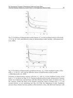
The literature offers ample coverage of the results for thermoaerodynamic characteristics of
bundles of tubes with cut fins (Taranyan et al., 1972; Kuntysh & Iokhvedov, 1968; Antufiev
& Gusyev, 1968; Iokhvedov et al., 1975; Antufiev, 1965) (Fig. 1). Such heat transfer surfaces
are fabricated from the tubes with a typical helical finning by cutting the fins into short
sections by a thin mill along the generatrix of a carrying cylinder or along a helical line at an
angle of 45
o
. Cutting does not practically diminish the fin surface and, according to data of
the above-mentioned works, enhances heat transfer by 12-36% depending on the fin
parameters and the method of cutting fins. The effect of flow turbulization, produced in this
case, is the more appreciable, the higher are the cut fins. However, in all cases an increase in
aerodynamic drag markedly outstrips an increase in heat transfer which on the whole
noticeably reduces the total effect of heat transfer enhancement. Besides, the production of
tubes with cut fins requires additional technological operations, which, in conjunction with

Heat Analysis and Thermodynamic Effects

160
a high susceptibility to contamination of the heat transfer surfaces from such tubes and
complexity of their cleaning, substantially limited their application.


Fig. 1. Tubes with cut fins (Taranyan et al., 1972; Kuntysh & Iokhvedov, 1968; Iokhvedov

et al., 1975)
More technologically advantageous, with similar characteristics of thermoaerodynamic
efficiency, is a solution involving the application of flow-agitating notches on the ends of
rolled-on fins (Kokorev et al., 1978; Kuntysh & Piir, 1991; Kuntysh, 1993), owing to which it
found use in manufacturing heat transfer surfaces from aluminum tubes for some air
cooling devices. However, this situation, apart from the limited range of application as to
temperature conditions, retained essential operational drawbacks of the cut fins with bent
edges, viz. an increased susceptibility to contamination and complexity of cleaning the
interfin gaps, aggravated by their considerable blocking by the deformed fin edges.
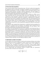
Fairly well-known is the type of finning referred to in the literature as segment finning
(Fig. 2). Judging from advertizing materials and from data (Weierman, 1976), such finning
can produce an appreciable effect even in the case of some loss by heat transfer surface in
comparison with continuous fins with the same height, thickness and pitch. Heat transfer is
enhanced here not only because of a decrease in the boundary layer thickness as a result of a
small width of an individual “segment” and the turbulization of flow on its separation from
sharp edges of the fin but also because each individual element of the segment fin is, in
essence, a straight rectangular fin with efficiency higher than of a disk fin. Estimates
according to data (Weierman, 1976) manifest that replacing a typical helical finning by
segment finning, with other conditions being equal, can decrease the number of tubes in a
bundle by 18-20%. However, reviewing the structures of present-day heat exchangers,
including power devices, indicates that, regardless of the above-stated assets that are
combined with easier manufacturability (the segment finning is formed by welding a
preliminarily notched steel strip to the tube by high-frequency currents), the considered
type of the intensified heat transfer surface has not found wide application as yet. This fact
is to some extent linked with a scanty investigation of thermoaerodynamic characteristics of
the surfaces from tubes with segment finning. Insufficiently reliable, by our data, are design
equations forming the basis for estimating thermoaerodynamic characteristics of the
bundles of such tubes.

Fig. 2. Segmented fins (Weierman, 1976)

Enhancement of Heat Transfer in the Bundles of Transversely-Finned Tubes


161
The enhancement method, described in (Fiebig et al., 1990), also involves perforation of a thin
fin. Its essence lies in the formation, on a rectangular fin behind the carrying cylinder, of two
delta wings representing bent parts of the perforated fin. The wings, inclined toward the
incident flow, generate longitudinal vortices enhancing transfer in the near-wall region, which,
with reference to actual heat exchangers, in the authors’ opinion, can increase heat transfer by
20% and decrease operational expenditure by 10%. These estimates, relying on the exploration
of experimental data for a single finned cylinder to a multirow heat exchanger, are too
optimistic, considering the variation in the flow turbulence over the depth of a finned bundle.
Study (Kuntysh & Kuznetsov, 1992) attributes the improvement of mass and dimensional
characteristics of the surfaces, made from circular tubes with a helical rolled-on finning, to
the removal of a finned part lying in the wake region behind the carrying cylinder, where
the heat transfer rate on the whole, as is well known, is relatively low. For the removal of the
finned part to be possibly more adaptable to manufacture, the authors suggest that fins
should be cut off on the chord along the plane parallel to the tube midsection (Fig. 3).
According to data (Kuntysh & Kuznetsov, 1992), the heat transfer coefficients, related to a
total surface of the tubes with a finning cutoff in the indicated fashion throughout height h,
increase in comparison with the case of typical finned tubes by 1.23 times at Re = 3·10
3
and
by 1.3 times at Re = 2.5·10
4
. Here, the aerodynamic drag is practically unchangeable.
However, due to the decrease in the area of the heat transfer surface, a total heat extraction
diminishes by 13% and 23%, respectively. Nonetheless, the authors assert that, with other
conditions being equal, up to 28% of the metal consumed for the finning fabrication can thus

be saved. Overall, the above-considered way of perfecting transversely finned surfaces
cannot be recognized as rational for obvious reasons.
Yet another trend for improving thermoaerodynamic characteristics of the tubular
transversely finned surfaces that involves a change of their geometry is a search for new
types of the arrangement of finned tube bundles. Main ideas of such developmental works
have been mostly borrowed from studies (Yevenko & Anisin, 1976;
Lokshin et al., 1982;
Migai & Firsova, 1986) conducted with smooth tube bundles. Among them are:
- a so-called crossed or lattice arrangement of the tubes;
- arrangements intermediate between purely in-line and purely staggered that can be
produced by changing the angle between the axes of longitudinal rows of ordinary in-
line tube bundles and the velocity vector of the incident flow;
- zigzag arrangements formed by an alternating longitudinal displacement of the tubes in
transverse rows of staggered bundles (Fig. 4); and
- bundles with an unequal number of tubes in transverse row.
A significant volume of investigations in these directions has been conducted in works
(Kuntysh & Kuznetsov, 1992; Kuntysh et al., 1991; Kuntysh & Stenin, 1993; Stenin, 1994;
Kuntysh et al., 1990).


Fig. 3. Tubes with finning cut off in the rear part

Heat Analysis and Thermodynamic Effects

162
When characterizing the results for thermoaerodynamic characteristics of crossed bundles it
should be noted that, in conformity with data (Kuntysh & Kuznetsov, 1992), such
arrangements do not enhance heat transfer in comparison with an ordinary layout of finned
tubes, although the drag decreases somewhat, and should in all probability be regarded as
inexpedient.

Studying the characteristics of intermediate in-line – staggered arrangements (Kuntysh &
Stenin, 1993; Stenin, 1994) revealed the effect of heat transfer enhancement reaching 5%
relative to the data for the original purely staggered bundle with a dense distribution of
tubes, which is comparable with an error of the experiments of this kind. An appreciably
greater effect can be attained, as study (Pis’mennyi, 1991) showed, using normal staggered
arrangements with optimal pitch relationships.
The use of zigzag arrangements can be justified to some extent primarily because the frontal
width of a bundle can be diminished (Fig. 4). Discrepancy of the data (Kuntysh &
Kuznetsov, 1992) allows us to assume that there is no noticeable effect of heat transfer
enhancement when the tubes in transverse rows of staggered bundles are displaced. The
matter is that, in the above-mentioned study, in experiments with zigzag tube bundles with
the fin factor ψ = 12.05 and with the drag equal to that of original ordinary staggered
bundles heat transfer increased by 8-17% and experiments with zigzag tube bundles with
the fin factor ψ = 17.5 indicated a decrease in the surface-average heat transfer. It is very
doubtful that the recorded relatively insignificant variation in the parameters can lead to a
substantial change in transfer in the bundles of transversely finned tubes. Obviously, the
above effects are linked with methodical errors of the experiments.


Fig. 4. Zigzag tube arrangement (Kuntysh & Kuznetsov, 1992)
Some studies (Kuntysh & Fedotova, 1983; Samie & Sparrow, 1986; Khavin, 1989)
considered the possibility of enhancing heat transfer by inclining the finned tubes with
respect to the direction of the incident flow. In this case, an additional turbulization of the
flow occurs as a result of its separation from the inlet edges of fins whose planes have a
positive attack angle. Experiments, performed in the region of Reynolds numbers Re =
5·10
3
- 5·10
4
with a single finned tube (Samie & Sparrow, 1986) and with staggered tube

bundles (Kuntysh & Fedotova, 1983), showed an increase the surface in average heat
transfer coefficients by 20-30% with an increase in the inclination angle by up to 40
o
. Here,
the most intense rise in α is observed for the inclination angles raging from 0 to 30
o
, which,
with a relatively monotonic increase in the aerodynamic drag, allows a selection of an
optimal inclination angle of the tubes.

Enhancement of Heat Transfer in the Bundles of Transversely-Finned Tubes


163
A certain reserve for increasing thermoaerodynamic efficiency of transversely finned tubes
resides in converting to a noncircular shape of the cross section of the fin-carrying tube.
Under definite conditions, specifically, with stringent limitations on the aerodynamic drag
of a heat exchanger, it is reasonable to use shaped (generally plane-oval or elliptical) tubes in
lieu of circular carrying tubes (Antufiev, 1966; Berman, 1965; Yudin & Fedorovich, 1992;
Ilgarubis et al., 1987). Geometric characteristics of such tube bundles include additional
parameters among which are the relation of longitudinal and lateral dimensions of the
cylinder cross section and the attack angle of the profile with respect to the direction of the
incident flow (Fig. 5). As works on heat transfer and aerodynamics of smooth and finned
shaped cylinders (Antufiev, 1966; Yudin & Fedorovich, 1992; Ilgarubis et al., 1987)
demonstrated, the search for optimal values of these parameters can be tied with the
prospects for improving the developed surfaces.


Fig. 5. Geometric characteristics of a plane-oval finned tube
In conclusion of the review part it should be noted that at the present time, in connection

with a significant increase in the metal cost for large volumes of the production of the heat
exchange equipment, it is considered expedient to use the ideas and designs leading to
decrease in the specific amount of metal per structure only by a few percent, with other
conditions being equal. Here, a good deal of attention is given to manufacturability of the
developed surfaces: their elements should be fabricated with the aid of waste-free high-
efficient technologies (like welding, rolling on and molding).
2. Physical substantiation of the proposed designs
In order to determine the ways of enhancement of local heat transfer in the bundles of
transversely finned tubes an experimental research of the effects of fin tube geometry, of
tube type, and of in-line and staggered arrangement on the distribution of heat transfer
coefficients over the fin surface was conducted in NTUU “Kiev Polytechnic Institute”.
In addition, the relationships governing local heat transfer incident to gas flows across
bundles of tubes with radial and helically-wound fins are of interest in calculating the
temperature distributions over the heating surfaces (especially at high loads), and in
determination of the real fin efficiencies E. The latter depend strongly upon the distribution
of heat transfer coefficients α over the fin surface, and are used in analytical engineering
methods for converting from convection to reduced values of heat transfer coefficients.
The measurement of the distribution of α over a fin involves great procedural difficulties, so
relatively little was done on this problem.
Here we present the results of the studies on the local heat transfer coefficients in tubes with
radial fins of different geometries, operating in various bundle arrangements.
d
1
d
2