Data Analysis Machine Learning and Applications Episode 1 Part 2 potx

54 Kamila Migdađ Najman and Krzysztof Najman
itself
6
. Since the learning algorithm of the SOM network is not deterministic, in
subsequent iterations it is possible to obtain a network with very weak discriminating
properties. In such a situation the value of the Silhouette index in subsequent stages
of variable reduction may not be monotone, what would make the interpretation
of obtained results substantially more difficult. At the end it is worth to note that
for large databases the repetitive construction of the SOM networks may be time
consuming and may require a large computing capacity of the computer equipment
used.
In the opinion of the authors the presented method proved its utility in numerous
empirical studies and may be successfully applied in practice.
References
DEBOECK G., KOHONEN T. (1998), Visual explorations in finance with Self-Organizing
Maps, Springer-Verlag, London.
GNANADESIKAN R., KETTENRING J.R., TSAO S.L. (1995), Weighting and selection of
variables for cluster analysis, Journal of Classification, vol. 12, p. 113-136.
GORDON A.D. (1999), Classification , Chapman and Hall / CRC, London, p.3
KOHONEN T. (1997), Self-Organizing Maps, Springer Series in Information Sciences,
Springer-Verlag, Berlin Heidelberg.
MILLIGAN G.W., COOPER M.C. (1985), An examination of procedures for determining the
number of clusters in data set. Psychometrika, 50(2), p. 159-179.
MILLIGAN G.W. (1994), Issues in Applied Classification: Selection of Variables to Cluster,
Classification Society of North America News Letter, November Issue 37.
MILLIGAN G.W. (1996), Clustering validation: Results and implications for applied analy-
ses. In Phipps Arabie, Lawrence Hubert & G. DeSoete (Eds.), Clustering and classifica-
tion, River Edge, NJ: World Scientific, p. 341-375.
MIGDAĐ NAJMAN K., NAJMAN K. (2003), Zastosowanie sieci neuronowej typu SOM w
badaniu przestrzennego zró
˙

znicowania powiatów, Wiadomo
´
sci Statystyczne, 4/2003, p.
72-85.
ROUSSEEUW P.J. (1987), Silhouettes: a graphical aid to the interpretation and validation of
cluster analysis. J. Comput. Appl. Math. 20, p. 53-65.
VESANTO J. (1997), Data Mining Techniques Based on the Self Organizing Map, Thesis for
the degree of Master of Science in Engineering, Helsinki University of Technology.
6
The quality of the SOM network is assessed on the basis of the following coefficients:
topographic, distortion and quantisation.
Calibrating Margin–based Classifier Scores into
Polychotomous Probabilities
Martin Gebel
1
and Claus Weihs
2
1
Graduiertenkolleg Statistische Modellbildung,
Lehrstuhl für Computergestützte Statistik,
Universität Dortmund, D-44221 Dortmund, Germany

2
Lehrstuhl für Computergestützte Statistik,
Universität Dortmund, D-44221 Dortmund, Germany

Abstract. Margin–based classifiers like the SVM and ANN have two drawbacks. They are
only directly applicable for two–class problems and they only output scores which do not
reflect the assessment uncertainty. K–class assessment probabilities are usually generated by
using a reduction to binary tasks, univariate calibration and further application of the pairwise

coupling algorithm. This paper presents an alternative to coupling with usage of the Dirichlet
distribution.
1 Introduction
Although many classification problems cover more than two classes, the margin–
based classifierssuchastheSupport Vector Machine (SVM)andArtificial Neural
Networks (ANN), are only directly applicable to binary classification tasks. Thus,
tasks with number of classes K greater than 2 require a reduction to several binary
problems and a following combination of the produced binary assessment values to
just one assessment value per class.
Before this combination it is beneficial to generate comparable outcomes by cali-
brating them to probabilities which reflect the assessment uncertainty in the binary
decisions, see Section 2. Analyzes for calibration of dichotomous classifier scores
show that the calibrators using Mapping with Logistic Regression or the Assign-
ment Value idea are performing best and most robust, see Gebel and Weihs (2007).
Up to date, pairwise coupling by Hastie and Tibshirani (1998) is the standard ap-
proach for the subsequent combination of binary assessment values, see Section 3.
Section 4 presents a new multi–class calibration method for margin–based classifiers
which combines the binary outcomes to assessment probabilities for the K classes.
This method based on the Dirichlet distribution will be compared in Section 5 to the
coupling algorithm.
30 Martin Gebel, Claus Weihs
2 Reduction to binary problems
Regard a classification task based on training set T :=
{
(x
i
,c
i
),i = 1, ,N
}

with x
i
being the ith observation of random vector X of p feature variables and respective
class c
i
∈C = {1, ,K}which is the realisation of random variableC determined by
a supervisor. A classifier produces an assessment value or score S
METHOD
(C = k|x
i
) for
every class k ∈
C and assigns to the class with highest assessment value. Some clas-
sification methods generate assessment values P
METHOD
(C = k|x
i
) which are regarded
as probabilties that represent the assessment uncertainty. It is desirable to compute
these kind of probabilities, because they are useful in cost–sensitive decisions and
for the comparison of results from different classifiers.
To generate assessment values of any kind, margin–based classifiers need to re-
duce multi–class tasks to seveal binary classfication problems. Allwein et al. (2000)
generalize the common methods for reducing multi–class into B binary problems
such as the one–against–rest and the all–pairs approach with using so–called error–
correcting output coding (ECOC) matrices. The way classes are considered in a
particular binary task b ∈
{
1, ,B
}

is incorporated into a code matrix < with K
rows and B columns. Each column vector \
b
determines with its elements \
k,b
∈
{
−1,0,+1
}
the classes for the bth classification task. A value of \
k,b
= 0 implies
that observations of the respective class k are ignored in the current task b while −1
and +1 determine whether a class k is regarded as the negative and the positive class,
respectively.
One–against–rest approach
In the one–against–rest approach the number of binary classification tasks B is equal
to the number of classes K. Each class is considered once as positive while all the
remaining classes are labeled as negative. Hence, the resulting code matrix < is of
size K ×K, displaying +1 on the diagonal while all other elements are −1.
All–pairs approach
In the all–pairs approach one learns for every single pair of classes a binary task b in
which one class is considered as positive and the other one as negative. Observations
which do not belong to either of these classes are omitted in the learning of this
binary task. Thus, < is a K×

K
2

–matrix with each column b consisting of elements

\
k
1
,b
=+1and\
k
2
,b
= −1 corresponding to a distinct class pair (k
1
,k
2
) while all
the remaining elements are 0.
3 Coupling probability estimates
As described before, the reduction approaches apply to each column \
b
of the code
matrix <,i.e.binarytaskb, a classification procedure. Thus, the output of the reduc-
tion approach consists of B score vectors s
+,b
(x
i
) for the associated positive class.
Calibrating Margin–based Classifier Scores into Polychotomous Probabilities 31
To each set of scores separately one of the univariate calibration methods described
in Gebel and Weihs (2007) can be applied. The outcome is a calibrated assessment
probability p
+,b
(x

i
) which reflects the probabilistic confidence in assessing observa-
tion x
i
for task b to the set of positive classes K
b,+
:=

k;\
k,b
=+1

as opposed to
the set of negative classes K
b,−
:=

k;\
k,b
= −1

. Hence, this calibrated assessment
probability can be regarded as function of the assessment probabilities involved in
the current task:
p
+,b
(x
i
)=


k∈K
b,+
P(C = k|x
i
)

k∈K
b,+
∪K
b,−
P(C = k|x
i
)
. (1)
The values P(C = k|x
i
) solving equation (1) would be the assessment probabilities
that reflect the assessment uncertainty. However, considering the additional con-
straint to assessment probabilities
K

k=1
P(C = k|x
i
)=1(2)
there exist only K −1 free parameters P(C = k|x
i
) but at least K equations for the
one–against–rest approach and even more for all–pairs (K(K −1)/2). Since the num-
ber of free parameters is always smaller than the number of constraints, no unique

solution for the calculation of assessment probabilities is possible and an approxima-
tive solution has to be found instead. Therefore, Hastie and Tibshirani (1998) supply
the coupling algorithm which finds the estimated conditional probabilities ˆp
+,b
(x
i
)
as realizations of a Binomial distributed random variable with an expected value z
b,i
in a way that
•ˆp
+1,b
(x
i
) generate unique assessment probabilities
ˆ
P(C = k|x
i
),
•
ˆ
P(C = k|x
i
) meet the probability constraint (2) and
•ˆp
+1,b
(x
i
) have minimal Kullback–Leibler divergence to observed p
+1,b

(x
i
).
4 Dirichlet calibration
The idea underlying the following multivariate calibration method is to transform the
combined binary classification task outputs into realizations of a Dirichlet distributed
random vector P ∼
D(h
1
, ,h
K
) and regard the elements as assessment probabilities
P
k
:= P(C = k|x).
Due to the concept of well–calibration by DeGroot and Fienberg (1983), we want to
achieve that the confidence in the assignment to a particular class converges to the
probability for this class. This requirement can be easily attained with a Dirichlet
distributed random vector by choosing parameters h
k
proportional to the a–priori
probabilities S
1
, ,S
K
of classes, since elements P
k
have expected values E(P
k
)=

h
k
/

K
j=1
h
j
.
32 Martin Gebel, Claus Weihs
Dirichlet distribution
A random vector P =(P
1
, ,P
K
)

generated by
P
k
=
S
k

K
j=1
S
j
(k = 1,2, ,K)
with K independently F

2
–distributed random variables S
k
∼ F
2
(2 · h
k
) is Dirichlet
distributed with parameters h
1
, ,h
K
, see Johnson et al. (2002).
Dirichlet calibration
Initially, instead of applying a univariate calibration method we normalize the output
vectors s
i,+1,b
by dividing them by their range and add half the range so that boundary
values (s = 0) lead to boundary probabilities (p = 0.5):
p
i,+1,b
:=
s
i,+1,b
+ U·max
i
|s
i,+1,b
|
2·U ·max

i
|s
i,+1,b
|
, (3)
since the doubled maximum of absolute values of scores is the range of scores. It is
required to use a smoothing factor U = 1.05 in (3) so that p
i,+1,b
∈ ]0,1[, since we
calculate in the following the geometric mean of associated binary proportions for
each class k ∈
{
1, ,K
}
r
i,k
:=
⎡
⎣

b:\
k,b
=+1
p
i,+1,b
·

b:\
k,b
=−1

(1−p
i,+1,b
)
⎤
⎦
1
#
{
\
k,b
≡0
}
.
This mean confidence is regarded as a realization of a Beta distributed random vari-
able R
k
∼ B (D
k
,E
k
) and parameters D
k
and E
k
are estimated from the training set
by the method of moments. We prefer the geometric to the arithmetic mean of pro-
portions, since the product is well applicable for proportions, especially when they
are skewed. Skewed proportions are likely to occur when using the one–against–rest
approach in situations with high class numbers, since here the number of negative
strongly outnumber the positive class observations.

To derive a multivariate Dirichlet distributed random vector, the r
i,k
can be trans-
formed to realizations of a uniformly distributed random variable
u
i,k
:= F
B,
ˆ
D
k
,
ˆ
E
k
(r
i,k
) .
By using the inverse of the F
2
–distribution function these uniformly distributed ran-
dom variables are further transformed into F
2
–distributed random variables. The re-
alizations of a Dirichlet distributed random vector P ∼
D(h
1
, ,h
K
) with elements

ˆp
i,k
:=
F
−1
F
2
,h
k
(u
i,k
)

K
j=1
F
−1
F
2
,h
j
(u
i, j
)
Calibrating Margin–based Classifier Scores into Polychotomous Probabilities 33
are achieved by normalizing. New parameters h
1
, ,h
K
should be chosen propor-

tional to frequencies S
1
, ,S
K
of the particular classes. In the optimization proce-
dure we choose the factor m = 1,2, ,2·N with respective parameters h
k
= m ·S
k
which score highest on the training set in terms of performance, determined by the
geometric mean of measures (4), (5) and (6).
5 Comparison
This section supplies a comparison of the presented calibration methods based on
their performance. Naturally, the precision of a classification method is the major
characteristic of its performance. However, a comparison of classification and cal-
ibration methods just on the basis of the precision alone, results in a loss of infor-
mation and would not include all requirements a probabilistic classifier score has
to fulfill. To overcome this problem, calibrated probabilities should satisfy the two
additional axioms:
• Effectiveness in the assignment and
• Well–calibration in the sense of DeGroot and Fienberg (1983).
Precision
The correctness rate
Cr =
1
N
N

i=1
I

[ ˆc(x
i
)=c
i
]
(x
i
) (4)
where I is the indicator function, is the key performance measure in classification,
since it mirrors the quality of the assignment to classes.
Effective assignment
Assessment probabilities should be effective in their assignment, i. e. moderately
high for true classes and small for false classes. An indicator for such an effectiveness
is the complement of the Root Mean Squared Error:
1−RMSE := 1−
1
N
N

i=1




1
K
K

k=1


I
[c
i
=k]
(x
i
) −P(c
i
= k|x)

2
. (5)
Well–calibrated probabilities
DeGroot and Fienberg (1983) give the following definition of a well–calibrated fore-
cast: “If we forecast an event with probability p, it should occur with a relative fre-
quency of about p.” To transfer this requirement from forecasting to classification
we partition the training/test set according to the assignment to classes into K groups
T
k
:=
{
(c
i
,x
i
) ∈ T :ˆc(x
i
)=k
}
with N

T
k
:= |T
k
| observations. Thus, in a partition T
k
34 Martin Gebel, Claus Weihs
the forecast is class k.
Predicted classes can differ from true classes and the remaining classes j ≡ k can
actually occur in a partition T
k
. Therefore, we estimate the average confidence
Cf
k, j
:=
1
N
T
k

x
i
∈T
k
P(k|ˆc(x
i
)= j) for every class j in a partition T
k
. According to
DeGroot and Fienberg (1983) this confidence should converge to the average cor-

rectness Cr
k, j
:=
1
N
T
k

x
i
∈T
k
I
[c(x
i
)= j]
. The average closeness of these two measures
WCR := 1−
1
K
2
K

k=1
K

j=1


Cf

k, j
−Cr
k, j


(6)
indicates how well–calibrated the assessment probabilities are.
On the one hand, the minimizing ”probabilities“ for the RMSE (5) can be just the
class indicators especially if overfitting occurs in the training set. On the other hand,
vectors of the individual correctness values maximize the WCR (6). To overcome
these drawbacks, it is convenient to combine the two calibration measures by their
geometric mean to the calibration measure
Cal :=

(1−RMSE) ·WCR . (7)
Experiments
The following experiments are based on the two three–class data sets Iris and
balance–scale from the UCI ML–Repository as well as the four–class data set B3,
see Newman et al. (1998) and Heilemann and Münch (1996), respectively.
Recent analyzes on risk minimization show that the minimization of a risk based on
the hinge loss which is usually used in SVM leads to scores without any probability
information, see Zhang (2004). Hence, the L2–SVM, see Suykens and Vandewalle
(1999), with using the quadratic hinge loss function and thus squared slack variables
is preferred to standard SVM. For classification we used the L2–SVM with radial–
basis Kernel function and a Neural Network with one hidden layer, both with the
one–against–rest and the all–pairs approach. In every binary decision a separate 3–
fold cross–validation grid search was used to find optimal parameters.
The results of the analyzes with 10–fold cross–validation for calibrating L2–SVM
and ANN are presented in Tables 1–2, respectively.
Table 1 shows that for L2–SVM no overall best calibration method is available. For

the Iris data set all–pairs with mapping outperforms the other methods, while for B3
the Dirichlet calibration and the all–pairs method without any calibration are per-
forming best. Considering the balance–scale data set, no big differences according
to correctness occur for the calibrators.
However, comparing these results to the ones for ANN in Table 2 shows that the
ANN, except the all–pairs method with no calibration, yields better results for all
data sets.
Here, the one–against–rest method with usage of the Dirichlet calibrator outper-
forms all other methods for Iris and B3. Considering Cr and Cal for balance–scale,
Calibrating Margin–based Classifier Scores into Polychotomous Probabilities 35
Table 1. Results for calibrating L2–SVM–scores
Iris B3 balance
Cr Cal Cr Cal Cr Cal
P
all–pairs,no
0.853 0.497 0.720 0.536 0.877 0.486
P
all–pairs,map
0.940 0.765 0.688 0.656 0.886 0.859
P
all–pairs,assign
0.927 0.761 0.694 0.677 0.886 0.832
P
all–pairs,Dirichlet
0.893 0.755 0.720 0.688 0.888 0.771
P
1–v–rest,no
0.833 0.539 0.688 0.570 0.885 0.464
P
1–v–rest,map

0.873 0.647 0.682 0.563 0.878 0.784
P
1–v–rest,assign
0.867 0.690 0.701 0.605 0.885 0.830
P
1–v–rest,Dirichlet
0.880 0.767 0.726 0.714 0.880 0.773
Table 2. Results for calibrating ANN–scores
Iris B3 balance
Cr Cal Cr Cal Cr Cal
P
all–pairs,no
0.667 0.614 0.490 0.573 0.302 0.414
P
all–pairs,map
0.973 0.909 0.752 0.756 0.970 0.946
P
all–pairs,assign
0.960 0.840 0.771 0.756 0.954 0.886
P
all–pairs,Dirichlet
0.953 0.892 0.777 0.739 0.851 0.619
P
1–v–rest,no
0.973 0.618 0.803 0.646 0.981 0.588
P
1–v–rest,map
0.973 0.942 0.803 0.785 0.978 0.921
P
1–v–rest,assign

0.973 0.896 0.796 0.752 0.976 0.829
P
1–v–rest,Dirichlet
0.973 0.963 0.815 0.809 0.971 0.952
Table 3. Comparing to direct classification methods
Iris B3 balance
Cr Cal Cr Cal Cr Cal
P
ANN,1–v–rest,Dirichlet
0.973 0.963 0.815 0.809 0.971 0.952
P
LDA
0.980 0.972 0.713 0.737 0.862 0.835
P
QDA
0.980 0.969 0.771 0.761 0.914 0.866
P
Logistic Regression
0.973 0.964 0.561 0.633 0.843 0.572
P
tree
0.927 0.821 0.427 0.556 0.746 0.664
P
Naive Bayes
0.947 0.936 0.650 0.668 0.904 0.710
one–against–rest with mapping performs best, but with correctness just slightly bet-
ter than the Dirichlet calibrator.
Finally, the comparison of the one–against–rest ANN with Dirichlet calibration to
other direct classification methods in Table 3 shows that for Iris LDA and QDA are
the best classifiers, since the Iris variables are more or less multivariate normally dis-

tributed. Considering the two further data sets the ANN yields highest performance.
36 Martin Gebel, Claus Weihs
6 Conclusion
In conclusion it is to say that calibration of binary classification outputs is beneficial
in most cases, especially for an ANN with the all–pairs algorithm.
Comparing classification methods to each other, one can see that the ANN with one–
against–rest and Dirichlet calibration performs better than other classifiers, except
LDA and QDA on Iris. Thus, the Dirichlet calibration is a nicely performing alter-
native, especially for ANN. The Dirichlet calibration yields better results with usage
of one–against–all, since combination of outputs with their geometric mean is bet-
ter applicable in this case where outputs are all based on the same binary decisions.
Furthermore, the Dirichlet calibration has got the advantage that here only one opti-
mization procedure has to be computed instead of the two steps for coupling with an
incorporated univariate calibration of binary outputs.
References
ALLWEIN, E. L. and SHAPIRE, R. E. and SINGER, Y. (2000): Reducing Multiclasss to
Binary: A Unifying Approach for Margin Classifiers. Journal of Machine Learning Re-
search 1, 113–141.
DEGROOT, M. H. and FIENBERG, S. E. (1983): The Comparison and Evaluation of Fore-
casters. The Statistician 32, 12–22.
GEBEL, M. and WEIHS, C. (2007): Calibrating classifier scores into probabilities. In: R.
Decker and H. Lenz (Eds.): Advances in Data Analysis. Springer, Heidelberg, 141–148.
HASTIE, T. and TIBSHIRANI, R. (1998): Classification by Pairwise Coupling. In: M. I. Jor-
dan, M. J. Kearns and S. A. Solla (Eds.): Advances in Neural Information Processing
Systems 10. MIT Press, Cambridge.
HEILEMANN, U. and MÜNCH, J. M. (1996): West german business cycles 1963–1994: A
multivariate discriminant analysis. CIRET–Conference in Singapore, CIRET–Studien 50.
JOHNSON, N. L. and KOTZ, S. and BALAKRISHNAN, N. (2002): Continuous Multivariate
Distributions 1, Models and Applications, 2nd edition. John Wiley & Sons, New York.
NEWMAN, D.J. and HETTICH, S. and BLAKE, C.L. and MERZ, C.J. (1998): UCI Reposi-

tory of machine learning databases [ />MLRepository.html]. University of California, Department of Information and Computer
Science, Irvine.
SUYKENS, J. A. K. and VANDEWALLE, J. P. L. (1999): Least Squares Support Vector
Machine classifiers. Neural Processing Letters 9:3,93–300.
ZHANG, T. (2004): Statistical behavior and consitency of classification methods based on
convex risk minimization. Annals of Statistics 32:1, 56–85.
Classification with Invariant Distance Substitution
Kernels
Bernard Haasdonk
1
and Hans Burkhardt
2
1
Institute of Mathematics, University of Freiburg
Hermann-Herder-Str. 10, 79104 Freiburg, Germany

,
2
Institute of Computer Science, University of Freiburg
Georges-Köhler-Allee 52, 79110 Freiburg, Germany

Abstract. Kernel methods offer a flexible toolbox for pattern analysis and machine learn-
ing. A general class of kernel functions which incorporates known pattern invariances are
invariant distance substitution (IDS) kernels. Instances such as tangent distance or dynamic
time-warping kernels have demonstrated the real world applicability. This motivates the de-
mand for investigating the elementary properties of the general IDS-kernels. In this paper we
formally state and demonstrate their invariance properties, in particular the adjustability of
the invariance in two conceptionally different ways. We characterize the definiteness of the
kernels. We apply the kernels in different classification methods, which demonstrates various
benefits of invariance.

1 Introduction
Kernel methods have gained large popularity in the pattern recognition and machine
learning communities due to the modularity of the algorithms and the data repre-
sentations by kernel functions, cf. (Schölkopf and Smola (2002)) and (Shawe-Taylor
and Cristianini (2004)). It is well known that prior knowledge of a problem at hand
must be incorporated in the solution to improve the generalization results. We ad-
dress a general class of kernel functions called IDS-kernels (Haasdonk and Burkhardt
(2007)) which incorporates prior knowledge given by pattern invariances.
The contribution of the current study is a detailed formalization of their basic
properties. We both formally characterize and illustratively demonstrate their ad-
justable invariance properties in Sec. 3. We formalize the definiteness properties in
detail in Sec. 4. The wide applicability of the kernels is demonstrated in different
classification methods in Sec. 5.
38 Bernard Haasdonk and Hans Burkhardt
2 Background
Kernel methods are general nonlinear analysis methods such as the kernel princi-
pal component analysis, support vector machine, kernel perceptron, kernel Fisher
discriminant, etc. (Schölkopf and Smola (2002)) and (Shawe-Taylor and Cristianini
(2004)). The main ingredient in these methods is the kernel as a similarity measure
between pairs of patterns from the set
X .
Definition 1 (Kernel, definiteness). A function k :
X ×X → R which is symmetric
is called a kernel. A kernel k is called positive definite (pd), if for all n and all sets of
observations (x
i
)
n
i=1
∈ X

n
the kernel matrix K :=(k (x
i
,x
j
))
n
i, j=1
satisfies v
T
Kv ≥ 0
for all v ∈ R
n
. If this only holds for all v satisfying v
T
1 = 0, the kernel is called
conditionally positive definite (cpd).
We denote some particular l
2
-inner-product

·,·

and l
2
-distance

·−·

based ker-

nels by k
lin
(x,x

) :=

x,x


,k
nd
(x,x

) := −

x −x


E
for E ∈ [0,2], k
pol
(x,x

) :=
(1+J

x,x


)

p
,k
rbf
(x,x

) := e
−J

x−x


2
for p ∈IN , J ∈R
+
. Here, the linear k
lin
, poly-
nomial k
pol
and Gaussian radial basis function (rbf) k
rbf
are pd for the given param-
eter ranges. The negative distance kernel k
nd
is cpd (Schölkopf and Smola (2002)).
We continue with formalizing the prior knowledge about pattern variations and cor-
responding notation:
Definition 2 (Transformation knowledge). We assume to have transformation
knowledge for a given task, i.e. the knowledge of a set T = {t :
X → X } of trans-

formations of the object space including the identity, i.e. id ∈ T. We denote the set
of transformed patterns of x ∈
X as T
x
:= {t(x)|t ∈ T } which are assumed to have
identical or similar inherent meaning as x.
The set of concatenations of transformations from two sets T,T

is denoted as
T ◦T

.Then-fold concatenation of transformations t are denoted as t
n+1
:= t ◦t
n
,the
corresponding sets denoted as T
n+1
:= T ◦T
n
.Ifallt ∈ T are invertible, we denote
the set of inverted functions as T
−1
. We denote the semigroup of transformations
generated by T as
¯
T :=

n∈IN
T

n
. The set
¯
T induces an equivalence relation on X
by x ∼x

:⇔ there exist
¯
t,
¯
t

∈
¯
T such that
¯
t(x)=
¯
t

(x

). The equivalence class of x is
denoted with E
x
and the set of all equivalence sets is X /
∼
.
Learning targets can often be modeled as functions of several input objects, for
instance depending on the training data and the data for which predictions are re-

quired. We define the desired notion of invariance:
Definition 3 (Total Invariance). We call a function f :
X
n
→ H totally invariant
with respect to T, if for all patterns x
1
, ,x
n
∈ X and transformations t
1
, ,t
n
∈ T
holds f (x
1
, ,x
n
)= f(t
1
(x
1
), ,t
n
(x
n
)).
As the IDS-kernels are based on distances, we define:
Classification with Invariant Distance Substitution Kernels 39
Definition 4 (Distance, Hilbertian Metric). A function d : X ×X → R is called a

distance, if it is symmetric and nonnegative and has zero diagonal, i.e. d(x, x)=0.
A distance is a Hilbertian metric if there exists an embedding into a Hilbert space
) :
X →H such that d(x,x

)=

)(x) −)(x

)

.
So in particular the triangle inequality does not need to be valid for a distance
function in this sense. Note also that a Hilbertian metric can still allow d(x,x

)=0
for x = x

.
Assuming some distance function d on the space of patterns
X enables to incor-
porate the invariance knowledge given by the transformations T into a new dissimi-
larity measure.
Definition 5 (Two-Sided invariant distance). For a given distance d on the set
X
and some cost function : : T ×T → R
+
with :(t,t

)=0 ⇔ t = t


= id,wedefine
the two-sided invariant distance as
d
2S
(x,x

) := inf
t,t

∈T
d(t(x),t

(x

)) +O:(t,t

). (1)
For O = 0 the distance is called unregularized. In the following we exclude artifi-
cial degenerate cases and reasonably assume that lim
O→f
d
2S
(x,x

)=d(x,x

) for all
x,x


. The requirement of precise invariance is often too strict for practical problems.
The points within T
x
are sometimes not to be regarded as identical to x, but only as
similar, where the similarity can even vary over T
x
. An intuitive example is optical
character recognition, where the similarity of a letter and its rotated version is de-
creasing with growing rotation angle. This approximate invariance can be realized
with IDS-kernels by choosing O > 0.
With the notion of invariant distance we define the invariant distance substitution
kernels as follows:
Definition 6 (IDS-Kernels). For a distance-based kernel,i.e.k(x,x

)= f(

x −x


),
and the invariant distance measure d
2S
we call k
IDS
(x,x

) := f (d
2S
(x,x


)) its invari-
ant distance substitution kernel (IDS-kernel). Similarly, for an inner-product-based
kernel k, i.e. k(x,x

)= f(

x,x


),wecallk
IDS
(x,x

) := f (

x,x


O
) its IDS-kernel,
where O ∈
X is an arbitrary origin and a generalization of the inner product is given
by

x,x


O
:= −
1

2
(d
2S
(x,x

)
2
−d
2S
(x,O)
2
−d
2S
(x

,O)
2
).
The IDS-kernels capture existing approaches such as tangent distance or dynamic
time-warping kernels which indicates the real world applicability, cf. (Haasdonk
(2005)) and (Haasdonk and Burkhardt (2007)) and the references therein.
Crucial for efficient computation of the kernels is to avoid explicit pattern trans-
formations by using or assuming some additional structure on T. An important com-
putational benefit of the IDS-kernels must be mentioned, which is the possibility to
precompute the distance matrices. By this, the final kernel evaluation is very cheap
and ordinary fast model selection by varying kernel or training parameters can be
performed.
40 Bernard Haasdonk and Hans Burkhardt
3 Adjustable invariance
As first elementary property, we address the invariance. The IDS-kernels offer two

possibilities for controlling the transformation extent and thereby interpolating be-
tween the invariant and non-invariant case. Firstly, the size of T can be adjusted.
Secondly, the regularization parameter O can be increased to reduce the invariance.
This is summarized in the following:
Proposition 1 (Invariance of IDS-Kernels).
i) If T = {id} and d is an arbitrary distance, then k
IDS
= k.
ii) If all t ∈T are invertible, then distance-based unregularized IDS-kernels k
IDS
(·,x)
are constant on (T
−1
◦T)
x
.
iii) If T =
¯
T and
¯
T
−1
=
¯
T , then unregularized IDS-kernels are totally invariant with
respect to
¯
T.
iv) If d is the ordinary Euclidean distance, then lim
O→f

k
IDS
= k.
Proof. Statement i) is obvious from the definition, as d
2S
= d in this case. Simi-
larly, iv) follows as lim
O→f
d
2S
= d. For statement ii), we note that if x

∈ (T
−1
◦
T)
x
, then there exist transformations t,t

∈ T such that t(x)=t

(x

) and conse-
quently d
2S
(x,x

)=0. So any distance-based kernel k
IDS

is constant on this set
(T
−1
◦T )
x
. For proving iii) we observe that for
¯
t,
¯
t

∈
¯
T holds d
2S
(
¯
t(x),
¯
t

(x

)) =
inf
t,t

d(t(
¯
t(x)),t


(
¯
t

(x

))) ≥ inf
t,t

d(t(x),t

(x

)) = d
2S
(x,x

). Using the same argu-
mentation with
¯
t(x) for x,
¯
t
−1
for
¯
t and similar replacements for x

,

¯
t

yields
d
2S
(x,x

) ≥ d
2S
(
¯
t(x),
¯
t

(x

)), which gives the total invariance of d
2S
and thus for all
unregularized IDS-kernels.
Points i) to iii) imply that the invariance can be adjusted by the size of T . Point ii)
implies that the invariance occasionally exceeds the set T
x
. If for instance T is closed
with respect to inversions, i.e. T = T
−1
, then the set of constant values is (T
2

)
x
. Point
iii) and iv) indicate that O can be used to interpolate between the full invariant and
non-invariant case.
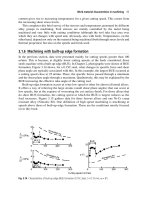
We give simple illustrations of the proposed kernels and these adjustability mech-
anisms in Fig. 1. For the illustrations, our objects are simply points in two dimen-
sions and several transformations define sets of points to be regarded as similar. We
fix one argument x

(denoted with a black dot) of the kernel, and the other argument
x is varying over the square [−1,2]
2
in the Euclidean plane. We plot the different
resulting kernel values k(x,x

) in gray-shades. All plots generated in the sequel can
be reproduced by the MATLAB library KerMet-Tools (Haasdonk (2005)).
In Fig. 1 a) we focus on a linear shift along a certain slant direction while in-
creasing the transformation extent, i.e. the size of T.Thefigure demonstrates the
behaviour of the linear unregularized IDS-kernel, which perfectly aligns to the trans-
formation direction as claimed by Prop. 1 i) to iii). It is striking that the captured
transformation range is indeed much larger than T and very accurate for the IDS-
kernels as promised by Prop. 1 ii).
The second means for controlling the transformation extent, namely increasing
the regularization parameter O, is also applicable for discrete transformations such
Classification with Invariant Distance Substitution Kernels 41
a)
b)
Fig. 1. Adjustable invariance of IDS-kernels. a) Linear kernel k

lin
IDS
with invariance wrt. linear
shifts, adjustability by increasing transformation extent by the set T, O = 0, b) kernel k
rbf
IDS
with
combined nonlinear and discrete transformations, adjustability by increasing regularization
parameter O.
as reflections and even in combination with continuous transformations such as ro-
tations, cf. Fig. 1 b). We see that the interpolation between the invariant and non-
invariant case as claimed in Prop. 1 ii) and iv) is nicely realized. So the approach is
indeed very general concerning types of transformations, comprising discrete, con-
tinuous, linear, nonlinear transformations and combinations thereof.
4 Positive definiteness
The second elementary property of interest, the positive definiteness of the kernels,
can be characterized as follows by applying a finding from (Haasdonk and Bahlmann
(2004)):
Proposition 2 (Definiteness of Simple IDS-Kernels). The following statements are
equivalent: i) d
2S
is a Hilbertian metric
ii)k
nd
IDS
is cpd for all E ∈[0,2] iii) k
lin
IDS
is pd
iv) k

rbf
IDS
is pd for all J ∈R
+
v) k
pol
IDS
is pd for all p ∈ IN ,J ∈R
+
.
So the crucial property, which determines the (c)pd-ness of IDS-kernels is, whether
the d
2S
is a Hilbertian metric. A practical criterion for disproving this is a violation
of the triangle inequality. A precise characterization for d
2S
being a Hilbertian metric
is obtained from the following.
Proposition 3 (Characterization of d
2S
as Hilbertian Metric). The unregularized
d
2S
is a Hilbertian metric if and only if d
2S
is totally invariant with respect to
¯
T and
d
2S

induces a Hilbertian metric on X /
∼
.
42 Bernard Haasdonk and Hans Burkhardt
Proof. Let d
2S
be a Hilbertian metric, i.e. d
2S
(x,x

)=

)(x) −)(x

)

. For prov-
ing the total invariance wrt.
¯
T it is sufficient to prove the total invariance wrt. T
due to transitivity. Assuming that for some choice of patterns/transformations holds
d
2S
(x,x

) = d
2S
(t(x),t

(x


)) a contradiction can be derived: Note that d
2S
(t(x), x

)
differs from one of both sides of the inequality, without loss of generality the left
one, and assume d
2S
(x,x

) < d
2S
(t(x), x

). The definition of the two-sided distance
implies d
2S
(x,t(x)) = inf
t

,t

d(t

(x),t

(t(x))) = 0viat

:= t and t


= id.Bythe
triangle inequality, this gives the desired contradiction d
2S
(x,x

) < d
2S
(t(x), x

) ≤
d
2S
(t(x), x)+d
2S
(x,x

)=0 + d
2S
(x,x

). Based on the total invariance, d
2S
(·,x

)
is constant on each E ∈
X /
∼
:Forallx ∼ x


transformations
¯
t,
¯
t

exist such that
¯
t(x)=
¯
t

(x

).Sowehaved
2S
(x,x

)=d
2S
(
¯
t(x), x

)=d
2S
(
¯
t


(x

),x

)=d
2S
(x

,x

),i.e.
this induces a well defined function on
X /
∼
by
¯
d
2S
(E, E

) := d
2S
(x(E),x(E

)).Here
x(E) denotes one representative from the equivalence class E ∈
X /
∼
. Obviously,

¯
d
2S
is a Hilbertian metric. via
¯
)(E) := )(x(E)). The reverse direction of the proposition
is clear by choosing )(x) :=
¯
)(E
x
).
Precise statements for or against pd-ness can be derived, which are solely based on
properties of the underlying T and base distance d:
Proposition 4 (Characterization by d and T).
i) If T is too small compared to
¯
T in the sense that there exists x

∈
¯
T
x
,but
d(T
x
,T
x

) > 0, then the unregularized d
2S

is not a Hilbertian metric.
ii) If d is the Euclidean distance in a Euclidean space
X and T
x
are parallel affine
subspaces of
X then the unregularized d
2S
is a Hilbertian metric.
Proof. For i) we note that d(T
x
,T
x

)=inf
t,t

∈T
d(t(x),t

(x

)) > 0. So d
2S
is not totally
invariant with respect to
¯
T and not a Hilbertian metric due to Prop. 3. For statement
ii) we can define the orthogonal projection ) :
X → H :=(T

O
)
⊥
on the orthog-
onal complement of the linear subspace through the origin O, which implies that
d
2S
(x,x

)=d()(x),)(x

)) and all sets T
x
are projected to a single point )(x) in
(T
O
)
⊥
.Sod
2S
is a Hilbertian metric.
In particular, these findings allow to state that the kernels on the left of Fig. 1 are
not pd as they are not totally invariant wrt.
¯
T. On the contrary, the extension of the
upper right plot yields a pd kernel, as soon as T
x
are complete affine subspaces. So
these criteria can practically decide about the pd-ness of IDS-kernels.
If IDS-kernels are involved in learning algorithms, one should be aware of the

possible indefiniteness, though it is frequently no relevant disadvantage in practice.
Kernel principal component analysis can work with indefinite kernels, the SVM is
known to tolerate indefinite kernels and further kernel methods are developed that
accept such kernels. Even if an IDS-kernel can be proven by the preceding to be
non-(c)pd in general, for various kernel parameter choices or a given dataset, the
resulting kernel matrix can occasionally still be (c)pd.
Classification with Invariant Distance Substitution Kernels 43
a) b) c) d)
Fig. 2. Illustration of non-invariant (upper row) versus invariant (lower row) kernel meth-
ods. a) Kernel k-nn classification with k
rbf
and scale-invariance, b) kernel perceptron with
k
pol
of degree 2 and y-axis reflection-invariance, c) one-class-classification with k
lin
and sine-
invariance, d) SVM with k
rbf
and rotation invariance.
5 Classification experiments
For demonstration of the practical applicability in kernel methods, we condense the
results on classification with IDS-kernels from (Haasdonk and Burkhardt (2007)) in
Fig. 2. That study also gives summaries of real-world applications in the fields of
optical character recognition and bacteria-recognition.
A simple kernel method is the kernel nearest-neighbour algorithm for classifi-
cation. Fig. 2 a) is the result of the kernel 1-nearest-neighbour algorithm with the
k
rbf
and its scale-invariant k

rbf
IDS
kernel, where the scaling sets T
x
are indicated with
black lines. The invariance properties of the kernel function obviously transfer to the
analysis method by IDS-kernels.
Another aspect of interest is the convergence speed of online-learning algorithms
exemplified by the kernel perceptron. We choose two random point sets of 20 points
each lying uniformly distributed within two horizontal rectangular stripes indicated
in Fig. 2 b). We incorporate the y-axis reflection invariance. By a random data draw-
ing repeated 20 times, the non-invariant kernel k
pol
of degree 2 results in 21.00±6.59
update steps, while the invariant kernel k
pol
IDS
converges much faster after 11.55±4.54
updates. So the explicit invariance knowledge leads to improved convergence prop-
erties.
An unsupervised method for novelty detection is the optimal enclosing hyper-
sphere algorithm (Shawe-Taylor and Cristianini (2004)). As illustrated in Fig. 2 c)
we choose 30 points randomly lying on a sine-curve, which are interpreted as nor-
mal observations. We randomly add 10 points on slightly downward/upward shifted
curves and want these points to be detected as novelties. The linear non-invariant k
lin
44 Bernard Haasdonk and Hans Burkhardt
results in an ordinary sphere, which however gives an average of 4.75 ±1.12 false
alarms, i.e. normal patterns detected as novelties, and 4.35±0.93 missed outliers, i.e.
outliers detected as normal patterns. As soon as we involve the sine-invariance by the

IDS-kernel we consistently obtain 0.00 ±0.00 false alarms and 0.40 ±0.50 misses.
So explicit invariance gives a remarkable performance gain in terms of recognition
or detection accuracy.
We conclude the 2D experiments with the SVM on two random sets of 20 points
distributed uniformly on two concentric rings, cf. Fig. 2 d). We involve rotation in-
variance explicitly by taking T as rotations by angles I ∈[−S/2,S/2]. In the example
we obtain an average of 16.40 ±1.67 SVs (indicated as black points) for the non-
invariant k
rbf
case, whereas the IDS-kernel only returns 3.40 ±0.75 SVs. So there
is a clear improvement by involving invariance expressed in the model size. This is
a determining factor for the required storage, number of test-kernel evaluations and
error estimates.
6 Conclusion
We investigated and formalized elementary properties of IDS-kernels. We have
proven that IDS-kernels offer two intuitive ways of adjusting the total invariance
to approximate invariance until recovering the non-invariant case for various dis-
crete, continuous, infinite and even non-group transformations. By this they build a
framework interpolating between invariant and non-invariant machine learning. The
definiteness of the kernels can be characterized precisely, which gives practical cri-
teria for checking positive definiteness in applications.
The experiments demonstrate various benefits. In addition to the model-inherent
invariance, when applying such kernels, further advantages can be the convergence
speed in online-learning methods, model size reduction in SV approaches, or im-
provement of prediction accuracy. We conclude that these kernels indeed can be
valuable tools for general pattern recognition problems with known invariances.
References
HAASDONK, B. (2005): Transformation Knowledge in Pattern Analysis with Kernel Methods
- Distance and Integration Kernels. PhD thesis, University of Freiburg.
HAASDONK, B. and BAHLMANN, B. (2004): Learning with distance substitution kernels.

In: Proc. of 26th DAGM-Symposium. Springer, 220–227.
HAASDONK, B. and BURKHARDT, H. (2007): Invariant kernels for pattern analysis and
machine learning. Machine Learning, 68, 35–61.
SCHÖLKOPF, B. and SMOLA, A. J. (2002): Learning with Kernels: Support Vector Ma-
chines, Regularization, Optimization and Beyond. MIT Press.
SHAWE-TAYLOR, J. and CRISTIANINI, N. (2004): Kernel Methods for Pattern Analysis.
Cambridge University Press.
Comparison of Local Classification Methods
Julia Schiffner and Claus Weihs
Department of Statistics, University of Dortmund,
44221 Dortmund, Germany

Abstract. In this paper four local classification methods are described and their statistical
properties in the case of local data generating processes (LDGPs) are compared. In order to
systematically compare the local methods and LDA as global standard technique, they are
applied to a variety of situations which are simulated by experimental design. This way, it is
possible to identify characteristics of the data that influence the classification performances of
individual methods. For the simulated data sets the local methods on the average yield lower
error rates than LDA. Additionally, based on the estimated effects of the influencing factors,
groups of similar methods are found and the differences between these groups are revealed.
Furthermore, it is possible to recommend certain methods for special data structures.
1 Introduction
We consider four local classification methods that all use the Bayes decision rule.
The Common Components and the Hierarchical Mixture Classifiers, as well as Mix-
ture Discriminant Analysis (MDA), are based on mixture models. In contrast, the
Localized LDA (LLDA) relies on locally adaptive weighting of observations. Appli-
cation of these methods can be beneficial in case of local data generating processes
(LDGPs). That is, there is a finite number of sources where each one can produce
data of several classes. The local data generation by individual processes can be de-
scribed by local models. The LDGPs may cause, for example, a division of the data

set at hand into several clusters containing data of one or more classes. For such
data structures global standard methods may lead to poor results. One way to obtain
more adequate methods is localization, which means to extend global methods for
the purpose of local modeling. Both MDA and LLDA can be considered as localized
versions of Linear Discriminant Analysis (LDA).
In this paper we want to examine and compare some of the statistical properties of
the four methods. These are questions of interest: Are the local methods appropriate
to classification in case of LDGPs and do they perform better than global methods?
Which data characteristics have a large impact on the classification performances
and which methods are favorable to special data structures? For this purpose, in a
70 Julia Schiffner and Claus Weihs
simulation study the local methods and LDA as widely-used global technique are
applied systematically to a large variety of situations generated and simulated by ex-
perimental design.
This paper is organized as follows: First the four local classification methods are de-
scribed and compared. In section 3 the simulation study and its results are presented.
Finally, in section 4 a summary is given.
2 Local classification methods
2.1 Common Components Classifier – CC Classifier
The CC Classifier (Titsias and Likas (2001)) constitutes an adaptation of a radial ba-
sis function (RBF) network for class conditional density estimation with full sharing
of kernels among classes. Miller and Uyar (1998) showed that the decision func-
tion of this RBF Classifier is equivalent to the Bayes decision function of a classifier
where class conditional densities are modeled by mixtures with common mixture
components.
Assume that there are K given classes denoted by c
1
, ,c
K
. Then in the common

components model the conditional density for class c
k
is
f
T
(x|c
k
)=
G
CC

j=1
S
jk
f
T
j
(x| j) for k = 1, ,K, (1)
where T denotes the set of all parameters and S
jk
represents the probability P( j|c
k
).
The densities f
T
j
(x| j), j = 1, ,G
CC
, with T
j

denoting the corresponding parame-
ters, do not depend on c
k
. Therefore all class conditional densities are explained by
the same G
CC
mixture components.
This implicates that the data consist of G
CC
groups that can contain observations of
all K classes. Because all data points in group j are explained by the same density
f
T
j
(x| j) classes in single groups are badly separable. The CC Classifier can only
perform well if individual groups mainly contain data of a unique class. This is more
likely if the parameter G
CC
is large. Therefore the classification performance de-
pends heavily on the choice of G
CC
.
In order to calculate the class posterior probabilities the parameters T
j
and the pri-
ors S
jk
and P
k
:= P(c

k
) are estimated based on maximum likelihood and the EM
algorithm. Typically, f
T
j
(x| j) is a normal density with parameters T
j
= {z
j
,6
j
}.A
derivation of the EM steps for the gaussian case is given in Titsias and Likas (2001),
p. 989.
2.2 Hierarchical Mixture Classifier – HM Classifier
The HM Classifier (Titsias and Likas (2002)) can be considered as extension of the
CC Classifier. We assume again that the data consist of G
HM
groups. But addition-
ally, we suppose that within each group j, j = 1, ,G
HM
, there are class-labeled
Comparison of Local Classification Methods 71
subgroups that are modeled by the densities f
T
kj
(x|c
k
, j) for k = 1, ,K, where T
kj

are the corresponding parameters. Then the unconditional density of x is given by a
three-level hierarchical mixture model
f
T
(x)=
G
HM

j=1
S
j
K

k=1
P
kj
f
T
kj
(x|c
k
, j) (2)
with S
j
representing the group prior probability P( j) and P
kj
denoting the probability
P(c
k
| j). The class conditional densities take the form

f
T
k
(x|c
k
)=
G
HM

j=1
S
jk
f
T
kj
(x|c
k
, j) for k = 1, ,K, (3)
where T
k
denotes the set of all parameters corresponding to class c
k
. Here, the mix-
ture components f
T
kj
(x|c
k
, j) depend on the class labels c
k

and hence each class
conditional density is described by a separate mixture. This resolves the data repre-
sentation drawback of the common components model.
The hierarchical structure of the model is maintained when calculating the class pos-
terior probabilities. In a first step, the group membership probabilities P( j |x) are
estimated and, in a second step, based on
ˆ
P( j|x) estimates for S
j
, P
kj
and T
kj
are
computed. For calculating
ˆ
P( j|x) the EM algorithm is used. Typically, f
T
kj
(x|c
k
, j)
is the density of a normal distribution with parameters T
kj
= {z
kj
,6
kj
}. Details on
the EM steps in the gaussian case can be found in Titsias and Likas (2002), p. 2230.

Note that the estimate
ˆ
T
kj
is only provided if
ˆ
P
kj
 0. Otherwise, it is assumed that
group j does not contain data of class c
k
and the associated subgroup is pruned.
2.3 Mixture Discriminant Analysis – MDA
MDA (Hastie and Tibshirani (1996)) is a localized form of Linear Discriminant Anal-
ysis (LDA). Applying LDA is equivalent to using the Bayes rule in case of normal
populations with different means and a common covariance matrix. The approach
taken by MDA is to model the class conditional densities by gaussian mixtures.
Suppose that each class c
k
is artificially divided into S
k
subclasses denoted by c
kj
,
j = 1, ,S
k
, and define S :=

K
k=1

S
k
as total number of subclasses. The subclasses
are modeled by normal densities with different mean vectors z
kj
and, similar to LDA,
a common covariance matrix 6. Then the class conditional densities are
f
z
k
,6
(x|c
k
)=
S
k

j=1
S
jk
I
z
kj
,6
(x|c
k
,c
kj
) for k = 1, ,K, (4)
where z

k
denotes the set of all subclass means in class c
k
and S
jk
represents the prob-
ability P(c
kj
|c
k
). The densities I
z
kj
,6
(x|c
k
,c
kj
) of the mixture components depend
on c
k
. Hence, as in the case of the HM Classifier, the class conditional densities are
described by separate mixtures.
72 Julia Schiffner and Claus Weihs
Parameters and priors are estimated based on maximum likelihood. In contrast to the
hierarchical approach taken by the HM Classifier, the MDA likelihood is maximized
directly using the EM algorithm.
Let x ∈ R
p
. LDA can be used as a tool for dimension reduction by choosing a

subspace of rank p
∗
≤ min{p,K −1} that maximally separates the class centers.
Hastie and Tibshirani (1996), p. 160, show that for MDA a dimension reduction sim-
ilar to LDA can be achieved by maximizing the log likelihood under the constraint
rank{z
kj
} = p
∗
with p
∗
≤ min{p, S −1}.
2.4 Localized LDA – LLDA
The Localized LDA (Czogiel et al. (2006)) relies on an idea of Tutz and Binder
(2005). They suggest the introduction of locally adaptive weights to the training data
in order to turn global methods into observation specific approaches that build in-
dividual classification rules for all observations to be classified. Tutz and Binder
(2005) consider only two class problems and focus on logistic regression. Czogiel et
al. (2006) extend their concept of localization to LDA by introducing weights to the
n nearest neighbors x
(1)
, ,x
(n)
of the observation x to be classified in the training
data set. These are given as
w

x,x
(i)


= W



x
(i)
−x


d
n
(x)

(5)
for i = 1, ,n, with W representing a kernel function. The Euclidean distance
d
n
(x)=


x
(n)
−x


to the farthest neighbor x
(n)
denotes the kernel width. The ob-
tained weights are locally adaptive in the sense that they depend on the Euclidean
distances of x and the training observations x

(i)
.
Various kernel functions can be used. For the simulation study we choose the kernel
W
J
(y)=exp(−Jy) that was found to be robust against varying data characteristics by
Czogiel et al. (2006). The parameter J ∈ R
+
has to be optimized.
For each x to be classified we obtain the n nearest neighbors in the training data
and the corresponding weights w

x,x
(i)

, i = 1, ,n. These are used to compute
weighted estimates of the class priors, the class centers and the common covariance
matrix required to calculate the linear discriminant function. The relevant formulas
are given in Czogiel et al. (2006), p. 135.
3 Simulation study
3.1 Data generation, influencing factors and experimental design
In this work we compare the local classification methods in the presence of local data
generating processes (LDGPs). In order to simulate data for the case of K classes and
M LDGPs we use the mixture model
Comparison of Local Classification Methods 73
Table 1. The chosen levels, coded by -1 and 1, of the influencing factors on the classification
performances determine the data generating model (equation (6)). The factor PUVAR defines
the proportion of useless variables that have equal class means and hence do not contribute to
class separation.
factor level

influencing factor
model
−1 +1
LP number of LDGPs M 24
PLP prior probabilities of LDGPs
S
j
unequal equal
DLP distance between LDGP centers
z
kj
large small
CL number of classes K 36
PCL (conditional) prior probabilities of classes
P
kj
unequal equal
DCL distance between class centers
z
kj
large small
VAR number of variables z
kj
, 6
kj
412
PUVAR proportion of useless variables
z
kj
0% 25%

DEP dependency in the variables 6
kj
no yes
DND deviation from the normal distribution
T no yes
f
z,6
(x)=
M

j=1
S
j
K

k=1
P
kj
T

I
z
kj
,6
kj
(x|c
k
, j)

(6)

with z and 6 denoting the sets of all z
kj
and 6
kj
and priors S
j
and P
kj
.The jth LDGP
is described by the local model

K
k=1
P
kj
T

I
z
kj
,6
kj
(x|c
k
, j)

. The transformation
of the gaussian mixture densities by the function T allows to produce data from non-
normal mixtures. In this work we use the system of densities by Johnson (1949) to
generate deviations from normality in skewness and kurtosis. If T is the identity the

data generating model equals the hierarchical mixture model in equation (2) with
gaussian subgroup densities and G
HM
= M.
We consider ten influencing factors which are given in Table 1. These factors de-
termine the data generating model. For example the factor PLP,defining the prior
probabilities of the LDGPs, is related to S
j
in equation (6) (cp. Table 1). We fixtwo
levels for every factor, coded by −1 and +1, which are also given in Table 1. In
general the low level is used for classification problems which should be of lower
difficulty, whereas the high level leads to situations where the premises of some
methods are not met (e.g. nonnormal mixture component densities) or the learning
problem is more complicated (e.g. more variables). For more details concerning the
choice of the factor levels see Schiffner (2006).
We use a fractional factorial 2
10−3
-design with tenfold replication leading to 1280
runs. For every run we construct a training data set with 3000 and a test data set
containing 1000 observations.
3.2 Results
We apply the local classification methods and global LDA to the simulated data sets
and obtain 1280 test data error rates r
i
, i = 1, ,1280, for every method. The chosen
74 Julia Schiffner and Claus Weihs
Table 2. Bayes errors and error rates of all classification methods with the specified param-
eters and mixture component densities on the 1280 simulated test data sets. R
2
denotes the

coefficients of determination for the linear regressions of the classification performances on
the influencing factors in Table 1.
mixture component error rate
method parameters
densities
minimum mean maximum
R
2
Bayes error - - 0.000 0.026 0.193 -
LDA - - 0.000 0.148 0.713 0.901
CC M G
CC
= Mf
T
j
= I
z
j
,6
j
0.000 0.441 0.821 0.871
CC MK G
CC
= M ·Kf
T
j
= I
z
j
,6

j
0.000 0.054 0.217 0.801
LLDA J = 5, n = 500 -
0.000 0.031 0.207 0.869
MDA S
k
= M - 0.000 0.042 0.205 0.904
HM G
HM
= Mf
T
kj
= I
z
kj
,6
kj
0.000 0.036 0.202 0.892
parameters, the group and subgroup densities assumed for the HM and CC Classi-
fiers and the resulting test data error rates are given in Table 2. The low Bayes errors
(cp. also Table 2) indicate that there are many easy classification problems. For the
data sets simulated in this study, in general, the local classification methods perform
much better than global LDA. An exception is the CC Classifier with M groups,
CC M, which probably suffers from the common components assumption in com-
bination with the low number of groups. The HM Classifier is the most flexible of
the mixture based methods. The underlying model is met in all simulated situations
where deviations from normality do not occur. Probably for this reason the error rates
for the HM Classifier are lower than for MDA and the CC Classifiers.
In order to measure the influence of the factors in Table 1 on the classification per-
formances of all methods we estimate their main and interaction effects by linear

regressions of ln(odds(1 −r
i
)) = ln((1−r
i
)/r
i
) ∈ R, i = 1, ,1280, on the coded
factors. Then an estimated effect of 1, e.g. of factor DND, can be interpreted as an
increase in proportion of hit rate to error rate by e ≈2.7.
The coefficients of determination, R
2
, indicate a good fit of the linear models for
all classification methods (cp. Table 2), hence the estimated factor effects are mean-
ingful. The estimated main effects are shown in Figure 1. For the most important
factors CL, DCL and VAR they indicate that a small number of classes, a big distance
between the class centers and a high number of variables improve the classification
performances of all methods.
To assess which classification methods react similarly to changes in data character-
istics they are clustered based on the Euclidean distances in their estimated main
and interaction effects. The resulting dendrogram in Figure 2 shows that one group
is formed by the HM Classifier, MDA and LLDA which also exhibit similarities in
their theoretical backgrounds. In the second group there are global LDA and the lo-
cal CC Classifier with MK groups, CC MK. The factors mainly revealing differences
between CC M, which is isolated in the dendrogram, and the remaining methods are
CL, DCL, VAR and LP (cp. Figure 1). For the first three factors the absolute effects
for CC M are much smaller. Additionally, CC M is the only method with a positive
Comparison of Local Classification Methods 75
LDA
CC M
CC MK

LLDA
MDA
HM
estimated main e
ff
ect
Ŧ6
Ŧ4
Ŧ20
2 4 6
LP
PLP
DLP
CL
PCL
DCL
VAR
PUVAR
DEP
D
N
Fig. 1. Estimated main effects of the influenc-
ing factors in Table 1 on the classification per-
formances of all methods
CC M
LLDA
MDA
HM
LDA
CC MK

2468
1012
distance
Fig. 2. Hierarchical clustering of the classifi-
cation methods using average linkage based
on the estimated factor effects
estimated effect of LP, the number of LDGPs, which probably indicates that a larger
number of groups improves the classification performance (cp. the error rates of CC
MK in Table 2). The factor DLP reveals differences between the two groups found
in the dendrogram. In contrast to the remaining methods, for both CC Classifiers
as well as LDA small distances between the LDGP centers are advantageous. Local
modeling is less necessary, if the LDGP centers for individual classes are close to-
gether and hence, the global and common components based methods perform better
than in other cases.
Based on theoretical considerations, the estimated factor effects and the test data er-
ror rates, we can assess which methods are favorable to some special situations. The
estimated effects of factor LP and the error rates in Table 2 show that application of
the CC Classifier can be disadvantageous and is only beneficial in conjunction with
a big number of groups G
CC
which, however, can make the interpretation of the re-
sults very difficult. However, for large M, problems in the E step of the classical EM
algorithm can occur for the CC and the HM Classifiers in the gaussian case due to
singular estimated covariance matrices. Hence, in situations with a large number of
LDGPs MDA can be favorable because it yields low error rates and is insensible to
changes of M (cp. Figure 1), probably thanks to the assumption of a common covari-
ance matrix and dimension reduction.
A drawback of MDA is that the numbers of subclasses for all K classes have to be
specified in advance. Because of subgroup-pruning for the HM Classifier only one
parameter G

HM
has to be fixed.
If deviations from normality occur in the mixture components LLDA can be recom-
mended since, like CC M, the estimated effect of DND is nearly zero and the test
data error rates are very small. In contrast to the mixture based methods it is appli-
cable to data of every structure because it does not assume the presence of groups,
76 Julia Schiffner and Claus Weihs
subgroups or subclasses. On the other hand, for this reason, the results of LLDA are
less interpretable.
4 Summary
In this paper different types of local classification methods, based on mixture models
or locally adaptive weighting, are compared in case of LDGPs. For the mixture mod-
els we can distinguish the common components and the separate mixtures approach.
In general the four local methods considered in this work are appropriate to classifi-
cation problems in the case of LDGPs and perform much better than global LDA on
the simulated data sets. However, the common components assumption in conjunc-
tion with a low number of groups has been found very disadvantageous. The most
important factors influencing the performances of all methods are the numbers of
classes and variables as well as the distances between the class centers. Based on all
estimated factor effects we identified two groups of similar methods. The differences
are mainly revealed by the factors LP and DLP, both related to the LDGPs. For a
large number of LDGPs MDA can be recommended. If the mixture components are
not gaussian LLDA appears to be a good choice. Future work can consist in con-
sidering robust versions of the compared methods that can better deal, for example,
with deviations from normality.
References
CZOGIEL, I., LUEBKE, K., ZENTGRAF, M. and WEIHS, C. (2006): Localized Linear
Discriminant Analysis. In: R. Decker, H J. Lenz (Eds.): Advances in Data Analysis.
Springer, Berlin, 133–140.
HASTIE, T.J. and TIBSHIRANI, R. J. (1996): Discriminant Analysis by Gaussian Mixtures.

Journal of the Royal Statistical Society B, 58, 155–176.
JOHNSON, N.L. (1949): Systems of Frequency Curves generated by Methods of Translation.
Biometrika, 36, 149–176.
MILLER, D. J. and UYAR, H. S. (1998): Combined Learning and Use for a Mixture Model
Equivalent to the RBF Classifier. Neural Computation, 10, 281–293.
SCHIFFNER, J. (2006): Vergleich von Klassifikationsverfahren für lokale Modelle. Diploma
Thesis, Department of Statistics, University of Dortmund, Dortmund, Germany.
TITSIAS, M. K. and LIKAS, A. (2001): Shared Kernel Models for Class Conditional Density
Estimation. IEEE Transactions on Neural Networks, 12(5), 987–997.
TITSIAS, M.K. and LIKAS, A. (2002): Mixtures of Experts Classification Using a Hierarchi-
cal Mixture Model. Neural Computation, 14, 2221–2244.
TUTZ, G. and BINDER H. (2005): Localized Classification. Statistics and Computing, 15,
155–166.