Data Analysis Machine Learning and Applications Episode 1 Part 4 pptx

22 Eugeniusz Gatnar
KW =
1
NM
2
N

i=1
L(x
i
)(M −L(x
i
)). (11)
Also Dietterich (2000) proposed the measure to assess the level of agreement
between classifiers. It is the kappa statistics:
N = 1 −
1
M

N
i=1
L(x
i
)(M −L(x
i
))
N(M −1) ¯p(1− ¯p)
. (12)
Hansen and Salamon (1990) introduced the measure of difficulty T. It is simply
the variance of the random variable Z = L(x)/M:
T = Var(Z). (13)

Two measures of diversity have been proposed by Partridge and Krzanowski
(1997) for evaluation of the software diversity. The first one is the generalized di-
versity measure:
GD = 1 −
p(2)
p(1)
, (14)
where p(k) is the probability that k randomly chosen classifiers will fail on the ob-
servation x. The second measure is named coincident failure diversity:
CFD =

0 where p
0
= 1
1
1−p
0

M
m=1
M−m
M−1
p
m
where p
0
< 1
, (15)
where p
m

is the probability that exactly m out of M classifiers will fail on an obser-
vation x.
4 Combination rules
Once we have produced the set of individual classifiers of desired level of diversity,
we combine their predictions to amplify their correct decisions and cancel out the
wrong ones. The combination function F in (1) depends on the type of the classifier
outputs.
There are three different forms of classifier output. The classifier can produce a
single class label (abstract level), rank the class labels according to their posterior
probabilities (rank level), or produce a vector of posterior probabilities for classes
(measurement level).
Majority voting is the most popular combination rule for class labels
1
:
ˆ
C
∗
(x)=argmax
j

M

m=1
I(
ˆ
C
m
(x)=l
j
)


. (16)
1
In the R statistical environment we obtain class labels using the command
predict( ,type="class")
.
Fusion of Multiple Statistical Classifiers 23
It can be proved that it is optimal if the number of classifiers is odd, they have the
same accuracy, and the classifier’s outputs are independent. If we have evidence that
certain models are more accurate than others, weighing the individual predictions
may improve the overall performance of the ensemble.
Behavior Knowledge Space developed by Huang and Suen (1995) uses a look-up
table that keeps track of how often each class combination is produced by the clas-
sifiers during training. Then, during testing, the winner class is the most frequently
observed class in the BKS table for the combination of class labels produced by the
set of classifiers.
Wernecke (1992) proposed a method similar to BKS, that uses the look-up table
with 95% confidence intervals of the class frequencies. If the intervals overlap, the
least wrong classifier gives the class label.
Naive Bayes combination introduced by Domingos and Pazzani (1997) also
needs training to estimate the prior and posterior probabilities:
s
j
(x)=P(l
j
)
M

m=1
P(

ˆ
C
m
(x)|l
j
). (17)
Finally, the class with the highest value of s
j
(x) is chosen as the ensemble prediction.
On the measurement level, each classifier produces a vector of posterior probabil-
ities
2
ˆ
C
m
(x)=[c
m1
(x),c
m2
(x), ,c
mJ
(x)]. And combining predictions of all models,
we have a matrix called decision profile for an instance x:
DP(x)=
⎡
⎣
c
11
(x) c
12

(x) c
1J
(x)

c
M1
(x) c
M2
(x) c
MJ
(x)
⎤
⎦
(18)
Based on the decision profile we calculate the support for each class (s
j
(x)), and
the final prediction of the ensemble is the class with the highest support:
ˆ
C
∗
(x)=argmax
j

s
j
(x)

. (19)
The most commonly used is the average (mean) rule:

s
j
(x)=
1
M
M

m=1
c
mj
(x). (20)
There are also other algebraic rules that calculate median, maximum, minimum and
product of posterior probabilities for the j-th class. For example, the product rule is:
s
j
(x)=
1
M
M

m=1
c
mj
(x). (21)
Kuncheva et al. (2001) proposed a combination method based on Decision Tem-
plates, that are averaged decision profiles for each class (DT
j
). Given an instance x,
2
We use the command

predict( ,type="prob")
.
24 Eugeniusz Gatnar
its decision profile is compared to the decision templates of each class, and the class
whose decision template is closest (in terms of the Euclidean distance) is chosen as
the ensemble prediction:
s
j
(x)=1−
1
MJ
M

m=1
J

k=1
(DT
j
(m,k)−c
mk
(x))
2
. (22)
There are other combination functions using more sophisticated methods, such
as fuzzy integrals (Grabisch, 1995), Dempster-Shafer theory of evidence (Rogova,
1994) etc.
The rules presented above can be divided into two groups: trainable and non-
trainable. In trainable rules we determine the values of their parameters using the
training set, e.g. cell frequencies in the BKS method, or Decision Templates for

classes.
5 Open problems
There are several problems that remain open in classifier fusion. In this paper we
only focus on two of them. We have shown above ten combination rules, so the
first problem is the search for the best one, i.e. the one that gives the more accurate
ensembles.
And the second problem is concerned with the relationship between diversity
measures and combination functions. If there is any, we would be able to predict the
ensemble accuracy knowing the level of diversity of its members.
6 Results of experiments
In order to find the best combination rule and determine relationship between com-
bination rules and diversity measures we have used 10 benchmark datasets, divided
into learning and test parts, as shown in Table 2.
For each dataset we have generated 100 ensembles of different sizes: M =
10,20, 30,40, 50, and we used classification trees
3
as the base models.
We have computed the average ranks for the combination functions, where rank
1 was for the best rule, i.e. the one that produced the most accurate ensemble, and
rank 10 - for the worst one. The ranks are presented in Table 3.
We found that the mean rule is simple and has consistent performance for the
measurement level, and majority voting is a good combination rule for class labels.
Maximum rule is too optimistic, while minimum rule is too pessimistic.
If the classifier correctly estimates the posterior probabilities, the product rule
should be considered. But it is sensitive to the most pessimistic classifier.
3
In order to grow trees, we have used the
Rpart
procedure written by Therneau and Atkinson
(1997) for the R environment.

Fusion of Multiple Statistical Classifiers 25
Table 2. Benchmark datasets.
Dataset Number of cases Number of cases Number of Number
in training set in test set predictors of classes
DNA 2124 1062 180 3
Letter 16000 4000 16 26
Satellite 4290 2145 36 6
Iris 100 50 4 3
Spam 3000 1601 57 2
Diabetes 512 256 8 2
Sonar 138 70 60 2
Vehicle 564 282 18 4
Soybean 455 228 34 19
Zip 7291 2007 256 10
Table 3. Average ranks for combination methods.
Method Rank
mean 2.98
vote 3.50
prod 4.73
med 4.91
min 6.37
bayes 6.42
max 7.28
DT 7.45
Wer 7.94
BKS 8.21
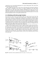
Figure 1 illustrates the comparison of performance of the combination functions
for the Spam dataset, which is typical of the datasets used in our experiments. We
can observe that the fixed rules perform better than the trained rules.
sred max min med prod vote bayes BKS Wer DT

0.06 0.08 0.10 0.12 0.14
Error
Fig. 1. Boxplots of combination rules for the Spam dataset.
26 Eugeniusz Gatnar
We have also noticed that the mean, median and vote rules give similar results.
Moreover, cluster analysis has shown that there are three more groups of rules of
similar performance: minimum and maximum, Bayes and Decision Templates, BKS
and Wernecke’s combination method.
In order to find the relationship between the combination functions and the di-
versity measures, we have calculated Pearson correlations. Correlations are moderate
(greater than 0.4) between mean, mode, product, and vote rules and Compound Di-
versity (6) as the only pairwise measure of diversity.
For non-pairwise measures correlations are strong (greater than 0.6) only be-
tween average, median, and vote rules, and Theta (13).
7 Conclusions
In this paper we have compared ten functions that combine outputs of the individual
classifiers into the ensemble. We have also studied the relationships between the
combination rules and diversity measures.
In general, we have observed that trained rules, such as BKS, Wernecke, Naive
Bayes and Decision Templates, perform poorly, especially for large number of com-
ponent classifiers (M). This result is contrary to Duin (2002), who argued that trained
rules are better than fixed rules.
We have also found that the mean rule and the voting rule are good for the mea-
surement level and abstract level, respectively.
But there are not strong correlations between the combination functions and the
diversity measures. This means that we can not predict the ensemble accuracy for
the particular combination method.
References
CUNNINGHAM, P. and CARNEY J. (2000): Diversity versus quality in classification en-
sembles based on feature selection, In: Proc. of the European Conference on Machine

Learning, Springer, Berlin, LNCS 1810, 109-116.
DIETTERICH, T.G. (2000): Ensemble methods in machine learning, In: Kittler J., Roli F.
(Eds.), Multiple Classifier Systems, Springer, Berlin, LNCS 1857, 1-15,
DOMINGOS, P. and PAZZANI, M. (1997): On the optimality of the simple Bayesian classifier
under zero- loss, Machine Learning, 29, 103-130.
DUIN, R. (2002): The Combining Classifier: Train or Not to Train?, In: Proc. of the 16th Int.
Conference on Pattern Recognition, IEEE Press.
GATNAR, E. (2005): A Diversity Measure for Tree-Based Classifier Ensembles. In: D. Baier,
R. Decker, and L. Schmidt-Thieme (Eds.): Data Analysis and Decision Support. Springer,
Heidelberg New York.
GIACINTO, G. and ROLI, F. (2001): Design of effective neural network ensembles for image
classification processes. Image Vision and Computing Journal, 19, 699–707.
GRABISCH M. (1995): On equivalence classes of fuzzy connectives -the case of fuzzy inte-
grals, IEEE Transactions on Fuzzy Systems, 3(1), 96-109.
Fusion of Multiple Statistical Classifiers 27
HANSEN, L.K. and SALAMON, P. (1990): Neural network ensembles. IEEE Transactions
on Pattern Analysis and Machine Intelligence 12, 993–1001.
HUANG, Y.S. and SUEN, C.Y. (1995): A method of combining multiple experts for the recog-
nition of unconstrained handwritten numerals, IEEE Transactions on Pattern Analysis
and Machine Intelligence, 17, 90-93.
KOHAVI, R. and WOLPERT, D.H. (1996): Bias plus variance decomposition for zero-one
loss functions, In: Saitta L. (Ed.), Machine Learning: Proceedings of the Thirteenth In-
ternational Conference, Morgan Kaufmann, 275- 283.
KUNCHEVA, L. and WHITAKER, C. (2003): Measures of diversity in classifier ensembles,
Machine Learning, 51, 181-207.
KUNCHEVA, L., WHITAKER, C., SHIPP, D. and DUIN, R. (2000): Is independence good
for combining classifiers? In: J. Kittler and F. Roli (Eds.): Proceedings of the First Inter-
national Workshop on Multiple Classifier Systems. LNCS 1857, Springer, Berlin.
KUNCHEVA, L., BEZDEK, J.C., and DUIN, R. (2001): Decision Templates for Multiple
Classifier Fusion: An Experimental Comparison. Pattern Recognition 34, 299-314.

PARTRIDGE, D. and YATES, W.B. (1996): Engineering multiversion neural-net systems.
Neural Computation 8, 869–893.
PARTRIDGE, D. and KRZANOWSKI, W.J. (1997): Software diversity: practical statistics for
its measurement and exploitation. Information and software Technology, 39, 707-717.
ROGOVA, (1994): Combining the results of several neural network classifiers, Neural Net-
works, 7, 777-781.
SKALAK, D.B. (1996): The sources of increased accuracy for two proposed boosting algo-
rithms. Proceedeings of the American Association for Artificial Intelligence AAAI-96,
Morgan Kaufmann, San Mateo.
THERNEAU, T.M. and ATKINSON, E.J. (1997): An introduction to recursive partitioning
using the RPART routines, Mayo Foundation, Rochester.
TUMER, K. and GHOSH, J. (1996): Analysis of decision boundaries in linearly combined
neural classifiers. Pattern Recognition 29, 341–348.
WERNECKE K D. (1992): A coupling procedure for discrimination of mixed data, Biomet-
rics, 48, 497-506.
Identification of Noisy Variables for Nonmetric and
Symbolic Data in Cluster Analysis
Marek Walesiak and Andrzej Dudek
Wroclaw University of Economics, Department of Econometrics and Computer Science,
Nowowiejska 3, 58-500 Jelenia Gora, Poland
{marek.walesiak, andrzej.dudek}@ae.jgora.pl
Abstract. A proposal of an extended version of the HINoV method for the identification of
the noisy variables (Carmone et al. (1999)) for nonmetric, mixed, and symbolic interval data is
presented in this paper. Proposed modifications are evaluated on simulated data from a variety
of models. The models contain the known structure of clusters. In addition, the models contain
a different number of noisy (irrelevant) variables added to obscure the underlying structure to
be recovered.
1 Introduction
Choosing variables is the one of the most important steps in a cluster analysis. Vari-
ables used in applied clustering should be selected and weighted carefully. In a clus-

ter analysis we should include only those variables that are believed to help to dis-
criminate the data (Milligan (1996), p. 348). Two classes of approaches, while choos-
ing the variables for cluster analysis, can facilitate a cluster recovery in the data (e.g.
Gnanadesikan et al. (1995); Milligan (1996), pp. 347–352):
– variable selection (selecting a subset of relevant variables),
– variable weighting (introducing relative importance of the variables according
to their weights).
Carmone et al. (1999) discussed the literature on the variable selection and
weighting (the characteristics of six methods and their limitations) and proposed the
HINoV method for the identification of the noisy variables, in the area of the variable
selection, to remedy problems with these methods. They demonstrated its robustness
with metric data and k-means algorithm. The authors suggest further studies of the
HINoV method with different types of data and other clustering algorithms on p.
508.
In this paper we propose extended version of the HINoV method for nonmetric,
mixed, and symbolic interval data. The proposed modifications are evaluated for
eight clustering algorithms on simulated data from a variety of models.
86 Marek Walesiak and Andrzej Dudek
2 Characteristics of the HINoV method and its modifications
Algorithm of Heuristic Identification of Noisy Variables (HINoV) method for metric
data (Carmone et al. (1999)) is following:
1. A data matrix [x
ij
] containing n objects and m normalized variables measured
on a metric scale (i = 1, ,n; j = 1, ,m) is a starting point.
2. Cluster, via
kmeans method, the observed data separately for each j-th variable
for a given number of clusters u. It is possible to use clustering methods based on
a distance matrix (
pam or any hierarchical agglomerative method: single, complete,

average, mcquitty, median, centroid, Ward).
3. Calculate adjusted Rand indices R
jl
( j,l = 1, , m) for partitions formed from
all distinct pairs of the m variables ( j = l). Due to a fact that adjusted Rand index is
symmetrical we need to calculate m(m −1)

2values.
4. Construct m×m adjusted Rand matrix (
parim). Sum rows or columns for each
j-th variable R
j•
=
m

l=1
R
jl
(topri):
Var ia ble
parim topri
⎡
⎢
⎢
⎢
⎣
M
1
M
2

.
.
.
M
m
⎤
⎥
⎥
⎥
⎦
⎡
⎢
⎢
⎢
⎣
R
12
R
1m
R
21
R
2m
.
.
.
.
.
.
.

.
.
.
.
.
R
m1
R
m2

⎤
⎥
⎥
⎥
⎦
⎡
⎢
⎢
⎢
⎣
R
1•
R
2•
.
.
.
R
m•
⎤

⎥
⎥
⎥
⎦
5. Rank
topri values R
1•
, R
2•
, , R
m•
in a decreasing order (stopri) and plot the
scree diagram. The size of the
topri values indicate a contribution of that variable to
the cluster structure. A scree diagram identifies sharp changes in the
topri values. Rel-
atively low-valued
topri variables (the noisy variables) are identified and eliminated
from the further analysis (say h variables).
6. Run a cluster analysis (based on the same classification method) with the se-
lected m −h variables.
The modification of the HINoV method for nonmetric data (where number of ob-
jects is much more than a number of categories) differs in steps 1, 2, and 6 (Walesiak
(2005)):
1. A data matrix [x
ij
] containing n objects and m ordinal and/or nominal variables
is a starting point.
2. For each j-th variable we receive natural clusters, where the number of clusters
equals the number of categories for that variable (for instance five for Likert scale or

seven for semantic differential scale).
6. Run a cluster analysis with one of clustering methods based on a distance
appropriate to nonmetric data (GDM2 for ordinal data – see Jajuga et al. (2003);
Sokal and Michener distance for nominal data) with the selected m −h variables.
The modification of the HINoV method for symbolic interval data differs in steps
1 and 2:
1. A symbolic data array containing n objects and m symbolic interval variables
is a starting point.
Identification of Noisy Variables for Nonmetric and Symbolic Data 87
2. Cluster the observed data with one of clustering methods (pam, single, com-
plete
, average, mcquitty, median, centroid, Ward) based on a distance appropriate to
the symbolic interval data (e.g. Hausdorff distance – see Billard and Diday (2006),
p. 246) separately for each j-th variable for a given number of clusters u.
Functions
HINoV.Mod and HINoV.Symbolic of clusterSim computer program
working in R allow adequately using mixed (metric, nonmetric), and the symbolic
interval data. The proposed modifications of the HINoV method are evaluated on
simulated data from a variety of models.
3 Simulation models
We generate data sets in eleven different scenarios. The models contain the known
structure of clusters. In the models 2-11 the noisy variables are simulated indepen-
dently from the uniform distribution.
Model 1. No cluster structure. 200 observations are simulated from the uniform
distribution over the unit hypercube in 10 dimensions (see Tibshirani et al [2001], p.
418).
Model 2. Two elongated clusters in 5 dimensions (3 noisy variables). Each clus-
ter contains 50 observations. The observations in each of the two clusters are inde-
pendent bivariate normal random variables with means (0, 0), (1, 5), and covariance
matrix


(V
jj
= 1, V
jl
= −0.9).
Model 3. Three elongated clusters in 7 dimensions (5 noisy variables). Each
cluster is randomly chosen to have 60, 30, 30 observations, and the observations are
independently drawn from bivariate normal distribution with means (0, 0), (1.5, 7),
(3, 14) and covariance matrix

(V
jj
= 1, V
jl
= −0.9).
Model 4. Three elongated clusters in 10 dimensions (7 noisy variables). Each
cluster is randomly chosen to have 70, 35, 35 observations, and the observations
are independently drawn from multivariate normal distribution with means (1.5, 6,
–3), (3, 12, –6), (4.5, 18, –9), and identity covariance matrix

, where V
jj
= 1
(1 ≤ j ≤ 3), V
12
= V
13
= −0.9, and V
23

= 0.9.
Model 5. Five clusters in 3 dimensions that are not well separated (1 noisy vari-
able). Each cluster contains 25 observations. The observations are independently
drawn from bivariate normal distribution with means (5, 5), (–3, 3), (3, –3), (0, 0),
(–5, –5), and identity covariance matrix

(V
jj
= 1, V
jl
= 0.9).
Model 6. Five clusters in 5 dimensions that are not well separated (2 noisy vari-
ables). Each cluster contains 30 observations. The observations are independently
drawn from multivariate normal distribution with means (5, 5, 5), (–3, 3, –3), (3, –3,
3), (0, 0, 0), (–5, –5, –5), and covariance matrix

, where V
jj
= 1(1≤ j ≤ 3),and
V
jl
= 0.9(1≤ j = l ≤ 3).
Model 7. Five clusters in 10 dimensions (8 noisy variables). Each cluster is ran-
domly chosen to have 50, 20, 20, 20, 20 observations, and the observations are inde-
pendently drawn from bivariate normal distribution with means (0, 0), (0, 10), (5, 5),
(10, 0), (10, 10), and identity covariance matrix

(V
jj
= 1, V

jl
= 0).
88 Marek Walesiak and Andrzej Dudek
Model 8. Five clusters in 9 dimensions (6 noisy variables). Each cluster contains
30 observations. The observations are independently drawn from multivariate normal
distribution with means (0, 0, 0), (10, 10, 10), (–10, –10, –10), (10, –10, 10), (–10,
10, 10), and identity covariance matrix

, where V
jj
= 3(1≤ j ≤ 3),andV
jl
= 2
(1 ≤ j = l ≤3).
Model 9. Four clusters in 6 dimensions (4 noisy variables). Each cluster is ran-
domly chosen to have 50, 50, 25, 25 observations, and the observations are indepen-
dently drawn from bivariate normal distribution with means (–4, 5), (5, 14), (14, 5),
(5, –4), and identity covariance matrix

(V
jj
= 1, V
jl
= 0).
Model 10. Four clusters in 12 dimensions (9 noisy variables). Each cluster con-
tains 30 observations. The observations are independently drawn from multivariate
normal distribution with means (–4, 5, –4), (5, 14, 5), (14, 5, 14), (5, –4, 5), and iden-
tity covariance matrix

, where V

jj
= 1(1≤ j ≤3),andV
jl
= 0(1≤ j = l ≤3).
Model 11. Four clusters in 10 dimensions (9 noisy variables). Each cluster con-
tains 35 observations. The observations on the first variable are independently drawn
from univariate normal distribution with means –2, 4, 10, 16 respectively, and iden-
tity variance V
2
j
= 0.5(1≤ j ≤ 4).
Ordinal data. The clusters in models 1-11 contain continuous data and a dis-
cretization process is performed on each variable to obtain ordinal data. The number
of categories k determines the width of each class intervals:

max
i
{x
ij
) −min
i
{x
ij
}

k. Independently for each variable each class interval re-
ceive category 1, ,k and the actual value of variable x
ij
is replaced by these cate-
gories. In simulation study k = 5 (for k = 7 we have received similar results).

Symbolic interval data. To obtain symbolic interval data the data were generated
for each model twice into sets A and B and minimal (maximal) value of

a
ij
,b
ij

is
treated as the beginning (the end) of an interval.
Fifty realizations were generated from each setting.
4 Discussion on the simulation results
In testing the robustness of the HINoV modified algorithm using simulated ordi-
nal or symbolic interval data, the major criterion was the identification of the noisy
variables. The HINoV-selected variables contain variables with the highest
topri val-
ues. In models 2-11 the number of nonnoisy variables is known. Due to this fact, in
simulation study, the number of the HINoV-selected variables equals the number of
nonnoisy variables in each model. When the noisy variables were identified, the next
step was to run the one of clustering methods based on distance matrix (
pam, single,
complete, average, mcquitty, median, centroid, Ward) with the nonnoisy subset of
variables (HINoV-selected variables) and with all variables. Then each clustering re-
sult was compared with the known cluster structure from models 2-11 using Hubert
and Arabie’s [1985] corrected Rand index (see Table 1 and 2).
Some conclusions can be drawn from the simulations results:
Identification of Noisy Variables for Nonmetric and Symbolic Data 89
Table 1. Cluster recovery for all variables and HINoV-selected subsets of variables for ordinal
data (five categories) by experimental model and clustering method
Model

Clustering method
pam ward single complete average mcquitty median centroid
2
a 0.38047 0.53576 0.00022 0.11912 0.42288 0.25114 0.00527 0.00032
b 0.84218 0.90705 0.72206 0.12010 0.99680 0.41796 0.30451 0.89835
3
a 0.27681 0.34071 0.00288 0.29392 0.40818 0.35435 0.04625 0.00192
b 0.85946 0.60606 0.36121 0.61090 0.68223 0.51487 0.49199 0.61156
4
a 0.35609 0.44997 0.00127 0.43860 0.53509 0.47083 0.04677 0.00295
b 0.83993 0.87224 0.56313 0.56541 0.80149 0.62102 0.54109 0.80156
5
a 0.54746 0.60139 0.27610 0.46735 0.58050 0.49842 0.33303 0.50178
b 0.91071 0.84888 0.48550 0.73720 0.81317 0.79644 0.72899 0.74462
6
a 0.61074 0.60821 0.13400 0.53296 0.61037 0.56426 0.35113 0.47885
b 0.83880 0.87183 0.56074 0.75584 0.86282 0.81395 0.71085 0.79018
7
a 0.10848 0.11946 0.00517 0.09267 0.10945 0.11883 0.00389 0.00659
b 0.80072 0.87399 0.27965 0.87892 0.94882 0.77503 0.74141 0.91638
8
a 0.31419 0.43180 0.00026 0.29529 0.40203 0.36771 0.00974 0.00023
b 0.95261 0.96372 0.58026 0.95596 0.96627 0.95507 0.93701 0.96582
9
a 0.37078 0.45915 0.01123 0.12128 0.50198 0.31134 0.04326 0.00709
b 0.99966 0.98498 0.93077 0.96993 0.99626 0.98024 0.95461 0.99703
10
a 0.29727 0.41152 0.00020 0.22358 0.41107 0.34663 0.00030 0.00007
b 1.00000 1.00000 0.99396 0.99911 1.00000 1.00000 0.99867 1.00000
¯

b
0.89378 0.88097 0.60858 0.73259 0.89642 0.76384 0.71212 0.85838
¯r 0.53130 0.44119 0.56066 0.44540 0.45403 0.39900 0.61883 0.74730
ccr 98.22% 98.00% 94.44% 90.67% 97.11% 89.56% 98.89% 98.44%
11 a 0.04335 0.04394 0.00012 0.04388 0.03978 0,03106 0,00036 0.00009
b 0.14320 0.08223 0.12471 0.08497 0.10373 0,12355 0,04626 0,06419
a (b) – values represent Hubert and Arabie’s adjusted Rand indices averaged over fifty repli-
cations for each model with all variables (with HINoV-selected variables); ¯r =
¯
b − ¯a; ccr –
corrected cluster recovery.
1. The cluster recovery that used only the HINoV-selected variables for ordinal
data (Table 1) and symbolic interval data (Table 2) was better than the one that used
all variables for all models 2-10 and each clustering method.
2. Among 450 simulated data sets (nine models with 50 runs) the HINoV method
was better (see ccr in Table 1 and 2):
– from 89.56% (mcquitty) to 98.89% (median) of runs for ordinal data,
– from 91.78% (ward) to 99,78% (centroid) of runs for symbolic interval data.
3. Figure 1 shows the relationship between the values of adjusted Rand indices
averaged over fifty replications and models 2-10 with the HINoV-selected variables
(
¯
b) and values showing an improvement (¯r) of average adjusted Rand indices (cluster
recovery with the HINoV selected variables against all variables) separately for eight
clustering methods and types of data (ordinal, symbolic interval). Based on adjusted
90 Marek Walesiak and Andrzej Dudek
Table 2. Cluster recovery for all variables and HINoV-selected subsets of variables for sym-
bolic interval data by experimental model and clustering method
Model
Clustering method

pam ward single complete average mcquitty median centroid
2
a 0.86670 0.87920 0.08006 0.28578 0.32479 0.49424 0.02107 0.00004
b 0.99920 0.97987 0.91681 0.99680 0.99524 0.98039 0.85840 0.95739
3
a 0.41934 0.39743 0.00368 0.37361 0.38831 0.36597 0.00088 0.00476
b 1.00000 1.00000 1.00000 1.00000 1.00000 1.00000 0.99062 1.00000
4
a 0.04896 0.01641 0.00269 0.01653 –0.00075 0.01009 0.00177 0.00023
b 1.00000 1.00000 1.00000 1.00000 1.00000 1.00000 1.00000 1.00000
5
a 0.71543 0.70144 0.73792 0.47491 0.60960 0.53842 0.34231 0.28338
b 0.99556 0.99718 0.98270 0.91522 0.99478 0.99210 0.90252 0.97237
6
a 0.75308 0.67237 0.33392 0.47230 0.67817 0.55727 0.18194 0.10131
b 0.99631 0.99764 0.99169 0.95100 0.98809 0.97881 0.84463 0.99866
7
a 0.36466 0.51262 0.00992 0.32856 0.33905 0.39823 0.00527 0.00681
b 1.00000 0.99974 1.00000 0.98493 0.99954 1.00000 0.99974 0.99954
8
a 0.74711 0.85104 0.01675 0.50459 0.51029 0.61615 0.00056 0.00023
b 1.00000 0.99966 0.99932 0.99966 0.99966 0.99843 0.99835 1.00000
9
a 0.86040 0.90306 0.30121 0.26791 0.54639 0.62620 0.00245 0.00419
b 1.00000 1.00000 1.00000 1.00000 1.00000 1.00000 1.00000 1.00000
10
a 0.70324 0.91460 0.00941 0.48929 0.47886 0.54275 0.00007 0.00004
b 1.00000 1.00000 1.00000 1.00000 1.00000 1.00000 1.00000 1.00000
¯
b

0.99900 0.99712 0.98783 0.98306 0.99747 0.99441 0.95491 0.99199
¯r 0.39023 0.34732 0.82166 0.62601 0.56687 0.53337 0.89310 0.94744
ccr 94.67% 91.78% 97.33% 99.11% 96.22% 96.44% 99.56% 99.78%
11
a 0.05334 0.04188 0.00007 0.03389 0.02904 0.03313 0.00009 0.00004
b 0.12282 0.04339 0.04590 0.08259 0.08427 0.14440 0.04380 0.08438
a (b);¯r =
¯
b − ¯a; ccr – see Table 1.
Rand indices averaged over fifty replications and models 2-10 the improvements in
cluster recovery (HINoV selected variables against all variables) are varying:
– for ordinal data from 0.3990 (mcquitty) to 0.7473 (centroid),
– for symbolic interval data from 0.3473 (ward) to 0.9474 (centroid).
5 Conclusions
The HINoV algorithm has limitations for analyzing nonmetric and symbolic interval
data almost the same as the ones mentioned in Carmone et al. (1999) article for
metric data.
First, the HINoV is of a little use with a nonmetric data set or a symbolic data
array in which all variables are noisy (no cluster structure – see model 1). In this
situation
topri values are similar and close to zero (see Table 3).
Identification of Noisy Variables for Nonmetric and Symbolic Data 91
0.3 0.4 0.5 0.6 0.7 0.8 0.9 1.0
0.6
0.7
0.8
0.9
1.0
r
b

pam
ward
single
complete
average
mcquitty
median
centroid
pam
ward
single
complete
average
mcquitty
median
centroid
ordinal data
symbolic data
Fig. 1. The relationship between values of
¯
b and ¯r
Source: own research
Table 3. Mean and standard deviation of
topri values for 10 variables in model 1
Va ri ab le
Ordinal data with five categories Symbolic data array
mean sd mean sd
1 –0.00393 0.01627 0.00080 0.02090
2 –0.00175 0.01736 0.00322 0.02154
3 0.00082 0.02009 0.00179 0.01740

4 –0.00115 0.01890 –0.00206 0.02243
5 0.00214 0.02297 –0.00025 0.02074
6 0.00690 0.02030 –0.00312 0.02108
7 –0.00002 0.02253 –0.00440 0.02044
8 0.00106 0.01754 0.00359 0.01994
9 0.00442 0.01998 0.00394 0.02617
10 –0.00363 0.01959 0.00023 0.02152
Second, the HINoV method depends on the relationship between pairs of vari-
ables. If we have only one variable with a cluster structure and the others are noisy,
the HINoV will not be able to isolate this nonnoisy variable (see Table 4).
Third, if all variables have the same cluster structure (no noisy variables) the
topri
values will be large and similar for all variables. The suggested selection process
using a scree diagram will be ineffective.
Fourth, an important problem is to decide on a proper number of clusters in stage
two of the HINoV algorithm with symbolic interval data. To resolve this problem we
should initiate the HINoV algorithm with a different number of clusters.
92 Marek Walesiak and Andrzej Dudek
Table 4. Mean and standard deviation of
topri values for 10 variables in model 11
Va ri ab le
Ordinal data with five categories Symbolic data array
mean sd mean sd
1 –0.00095 0.03050 0.00012 0.02961
2 –0.00198 0.02891 0.00070 0.03243
3 0.00078 0.02937 –0.00206 0.02969
4 –0.00155 0.02950 –0.00070 0.03185
5 0.00056 0.02997 –0.00152 0.03157
6 0.00148 0.03090 –0.00114 0.03064
7 –0.00246 0.02959 –0.00203 0.03019

8 –0.00274 0.03137 –0.00186 0.03021
9 –0.00099 0.02975 0.00088 0.03270
10 0.00023 0.02809 –0.00181 0.03126
References
BILLARD, L., DIDAY, E. (2006): Symbolic data analysis. Conceptual statistics and data
mining, Wiley, Chichester.
CARMONE, F.J., KARA, A. and MAXWELL, S. (1999): HINoV: a new method to improve
market segment definition by identifying noisy variables, Journal of Marketing Research,
vol. 36, November, 501-509.
GNANADESIKAN, R., KETTENRING, J.R., and TSAO, S.L. (1995): Weighting and selec-
tion of variables for cluster analysis, Journal of Classification, vol. 12, no. 1, 113-136.
HUBERT, L.J., ARABIE, P. (1985): Comparing partitions, Journal of Classification,vol.2,
no. 1, 193-218.
JAJUGA, K., WALESIAK, M., BAK, A. (2003): On the General Distance Measure, In:
M., Schwaiger, and O., Opitz (Eds.), Exploratory data analysis in empirical research,
Springer-Verlag, Berlin, Heidelberg, 104-109.
MILLIGAN, G.W. (1996): Clustering validation: results and implications for applied analyses,
In: P., Arabie, L.J., Hubert, G., de Soete (Eds.), Clustering and classification, World
Scientific, Singapore, 341–375.
TIBSHIRANI, R., WALTHER, G., HASTIE, T. (2001): Estimating the number of clusters in
a data set via the gap statistic, Journal of the Royal Statistical Society, ser. B, vol. 63, part
2, 411–423.
WALESIAK, M. (2005): Variable selection for cluster analysis – approaches, problems, meth-
ods, Plenary Session of the Committee on Statistics and Econometrics of the Polish
Academy of Sciences, 15, March, Wroclaw.
Incorporating Domain Specific Information into Gaia
Source Classification
Kester W. Smith, Carola Tiede and Coryn A.L. Bailer-Jones
Max–Planck–Institut für Astronomie,
Königstuhl 17, 69117 Heidelberg, Germany

Abstract. Astronomy is in the age of large scale surveys in which the gathering of multidi-
mensional data on thousands of millions of objects is now routine. Efficiently processing these
data - classifying objects, searching for structure, fitting astrophysical models - is a significant
conceptual (not to mention computational) challenge. While standard statistical methods, such
as Bayesian clustering, k-nearest neighbours, neural networks and support vector machines,
have been successfully applied to some areas of astronomy, it is often difficult to incorporate
domain specific information into these. For example, in astronomy we often have good phys-
ical models for the objects (e.g. stars) we observe. That is, we can reasonably well predict
the observables (typically, the stellar spectrum or colours) from the astrophysical parameters
(APs) we want to infer (such as mass, age and chemical composition). This is the “forward
model”: The task of classification or parameter estimation is then an inverse problem. In this
paper, we discuss the particular problem of combining astrometric information, effectively a
measure of the distance of the source, with spectroscopic information.
1 Introduction
Gaia is an ESA astronomical satellite that will be launched in 2011. Its mission is
to build a three dimensional map of the positions and velocities of a substantial part
of our galaxy. In addition to the basic position and velocity data, the astrophysical
nature of the detected objects will be determined. Since Gaia is expected to detect
upwards of a billion individual objects of various types, and since the mission will
not use an input catalogue, automated classification and parameterization based on
the dataset is a crucial part of the mission.
1.1 Astronomical context
From galactic rotation curves and other evidence it is believed that most material in
the universe is comprised of so-called dark matter. The nature of this material is a
fundamental current question in astronomy. The distribution and properties of the
dark matter at the time of the formation of our galaxy should leave traces in the dis-
tribution and dynamics of the stellar population that is observed today. Since heavy
78 Kester W. Smith, Carola Tiede and Coryn A.L. Bailer-Jones
elements are formed by nucleosynthesis in the centres of massive stars, and are there-

fore scarce at early epochs, their relative abundances in stellar atmospheres can be
used to discriminate between stellar populations on the basis of age. By building up
a complete picture of a large portion of our galaxy, such tracers of galactic evolution
can be studied in unprecedented detail.
1.2 Basic properties of the dataset
Gaia will detect all point sources down to a fixed limiting brightness. This limit corre-
sponds to the brightness of the Sun if observed at a distance of approximately 11,000
parsecs (35,000 light years, compared the accepted distance to the Galactic centre of
26,000 light years). The vast majority of detected sources will be stars, but the sam-
ple will also include several million galaxies and quasars, which are extragalactic
objects, and many objects from within our own solar system.
The positions of the various sources on the sky can of course be measured very
easily. Radial velocities are determined from Doppler shifts of spectral lines observed
with an onboard spectrometer. Transverse motions on the sky are of the order of a few
milliarcseconds per year, scaling with distance, and these motions must be mapped
over the timescale of the mission (5–6 years). Distances are a priori not known and
are in fact one of the most difficult, and most crucially important, measurements in
astronomy. Gaia is designed to measure the parallaxes of the stellar sources in order
to determine distances to nearby stars. The parallax in question is the result of the
changing viewpoint of the satellite as the Earth orbits the Sun. An object displaying
a parallax of one arcsecond relative to distant, negligable-parallax stars, has by defi-
nition a distance of 1 parsec (3.26 light years). This distance happens to correspond
roughly to the distance to the nearest stars. The parallax scales linearly with distance
so that the Sun at a distance of 11,000 parsec (the approximate brightness limit of
such an object for Gaia) would display a parallax of about 90 microarcseconds (zas)).
Gaia is designed to measure parallaxes with a standard error of around 25 zas, so that
the parallax-limit roughly corresponds to the brightness-limit for solar type stars.
As well as position, parallax and transverse motion (proper motion), and the high
resolution spectra used to determine the radial velocities, the Gaia satellite will return
low resolution spectra with approximately 96 resolution elements spanning the range

300-1000 nanometres (roughly from the ultraviolet to the near infrared range). These
spectra can be used to classify objects according to basic type (galaxies, quasars,
stars etc) and to then determine the basic parameters of the object (e.g. for stars, the
effective temperature of the atmosphere). This information is important because the
nature of the stellar population coupled with the kinematic information constrains
models of galaxy formation and evolution.
2 Classification and parametrization
As the sky is continuously scanned by the satellite’s detectors, sources are detected
on board and the data (position, low resolution spectra and high resolution spectrum)
Incorporating Domain Specific Information into Gaia Source Classification 79
are extracted from the raw detector output, processed into an efficient form and re-
turned to the ground station. As the mission proceeds, repeated visits to the same
area of sky allow the measurement of variations in the positions of sources, which
are used to build up a model of the proper motions and parallaxes for the full set
of sources. This leads to a distinction for the data processing between early mission
data, consisting of the spectra and positions, and late mission data, which includes
parallaxes and proper motions. The sources should be classified into broad astronom-
ical classes on the basis of the spectra alone in the early mission, and on the basis of
the spectra combined with astrometric information in the later part of the mission.
This classification is important for the astrophysics, but also for the astrometric so-
lution, since the distant quasars form a distant, essentially fixed (zero parallax and
zero proper motion, plus or minus measurement errors) population. The early mis-
sion classifier should feed back the identified extragalactic objects to the astrometric
processing, and the purer this sample, the better.
Once the classification is made, sources are fitted with astrophysical models to
recover various parameters, such as effective surface temperature or atmospheric el-
ement abundances for stars. The algorithms for this classification and regression are
in the early stages of development by the data processing consortium. For the classi-
fication, the algorithm mostly used at this stage is a Support Vector Machine (SVM)
after Vapnik (1995), taken from the library libSVM (Chang and Lin (2001)), with a

radial basis function (RBF) kernel. The decision to use SVM for classification is of
course provisional and other methods may be considered. Synthetic data for training
and testing the classifier is produced using standard models of various astronomical
source classes. The multi-class SVM used returns a probability vector containing the
probabilities that a particular source belongs to each class (Wu and Weng (2005)).
Sources are classified according to the highest component of the probability vector.
We are now incorporating into the simulated data values for the parallax and proper
motion, indicating a distance. The current task is to incorporate this information into
the classification and regression schemes.
3 Classification results
For current purposes, we consider only four classes of astrophysical object; single
stars and binary stars, both of which belong to the set of objects within our own
galaxy, and galaxies and quasars, both of which are extragalactic. Two datasets were
generated, each with a total of 5000 sources split evenly between the four classes
(i.e. 1250 of each). One set was used as a trianing set for the SVM, the other is a
test set from which the statistics are compiled. The classification results for the basic
SVM classifier running on the spectrum only are shown in Table 1. Here, and in
subsequent experiments, the input data are scaled to have mean of zero and standard
deviation of one for each bin. The classifier achieves an overall correct classification
rate of approximately 93%. The main confusion is between single stars and binaries.
The parallaxes of the simulated data for stars and quasars are shown in Figure 1.
The parallax could be included directly into the classifier as a 97th data point for each
80 Kester W. Smith, Carola Tiede and Coryn A.L. Bailer-Jones
Table 1. Confusion matrix for the SVM classifier, working on the spectral data without any
astrometric information. Reading row by row, the matrix shows the percentage of test sources
which are of a particular type, for example Stars, which are classified as each possible output
type. The leading diagonal shows the sources that are correctly classified (true positives). The
off-diagonal elements show the level of contamination (false positives) as a percentage of the
input source sample. In this test case, the numbers of each class of source were roughly equal
(just over 1000 each). In the real mission, the number of stars is expected to be three orders of

magnitude greater than the number of galaxies or quasars.
Stars Binaries Quasars Galaxies
Stars 88.21 9.27 2.43 0.09
Binaries 8.67 91.13 0.00 0.20
Quasars 2.04 0.90 95.77 1.28
Galaxies 0.00 0.00 0.62 99.38
Fig. 1. The distribution of simulated parallaxes for stars (filled squares) and quasars (+ signs).
object, alongside the 96 spectral bins. Such a classifier would be expected to perform
significantly better than spectrum-only version, and indeed it does (Table 2). It might,
however, be possible to include the parallax in the classification in a way that utilises
our knowledge of the astrophysical significance of the quantity. Significant values of
parallax are expected for a subset of the galactic sources, i.e. the stars and binaries.
Not all stars and binaries will have a detectable parallax, but none of the extragalactic
sources will. This then suggests a split in the data, based on parallax, into objects that
are certainly galactic and objects that may belong to any class.
To implement such a two-stage classifier, we trained two separate SVMs, one
with all four classes, and the other with the galactic sources (stars and binaries) only.
These SVMs were trained on the spectral data only, not including the parallax. We
then classified the entire test set with each classifier. For each object, the output from
each classifier is a four-component probability vector, in the case of the classifier
Incorporating Domain Specific Information into Gaia Source Classification 81
Table 2. Confusion matrix obtained by using the SVM with the parallax information included
as an additional input.
Stars Binaries Quasars Galaxies
Stars 93.52 6.03 0.45 0.00
Binaries 6.38 93.62 0.00 0.00
Quasars 0.76 0.14 98.91 0.19
Galaxies 0.00 0.00 0.41 99.59
trained only on galactic sources (stars and binaries), the probabilities for the quasars
and galaxies are necessarily always zero. Finally, we combined the output probability

vectors of the two SVMs using a weighting function based on the parallax value.
If P
1
and P
2
are the probability vectors for the galactic and general SVM classifier
respectively, they are combined to form the output probability as follows;
P = wP
1
+(1 −w)P
2
, (1)
w = 0.5(1 + tanh((D ×SNR)+G)) (2)
where SNR is the significance of the measured parallax, estimated by assuming that
the standard error is 25zas. The parameter D is set to 1. and the value of G to -5. With
these values, the function does not produce significant weighting (w ≈ 0.1) toward
exclusively galactic sources until the parallax rises to four times the standard error.
Fig. 2. The weighting function applied to the extragalactic sources.
The results of the two-stage classification are shown in Table 3. The leading
diagonal shows that the completeness at each class is not as good as in the case of
the single SVM classifier with parallax as discussed above (Table 2), however the
contamination of the extragalactic sources with misidentified galactic sources has
82 Kester W. Smith, Carola Tiede and Coryn A.L. Bailer-Jones
Fig. 3. The weighting function for the galactic sources. These sources are distributed through
a range of parallaxes.
been strongly reduced - in fact falling to zero for the test sample of 5000 objects.
As noted above, this is a significant advantage when the galaxies and quasars form
important classes for determining the astrometric solution, and when there will be
several hundred times more stars than extragalactic objects in the final sample.
Table 3. Confusion matrix obtained by using the SVM twice then combining the probabilities

weighted according to the value of the parallax.
Stars Binaries Quasars Galaxies
Stars 90.82 9.18 0.00 0.00
Binaries 8.87 91.13 0.00 0.00
Quasars 2.04 0.90 95.77 1.28
Galaxies 0.00 0.00 0.62 99.38
4 Summary
Since we know the relationship of the observables to the underlying nature of the
objects in the sample, we are in a position to incorporate this knowledge into the
classification or regression problems in an informed way, making maximum use of
this physical knowledge. The goal of this is twofold; Firstly, the addition of domain-
specific information should improve the predictive accuracy. Second, but not unim-
portant, is that it allows an interpretation of how the model works: the sensitivities
of the model observables to a given underlying parameter provide an explicit (and
Incorporating Domain Specific Information into Gaia Source Classification 83
unique) weighting function of the observables. Apart from making the model more
acceptable (and less like a “black box”), this allows us to identify where we gather
higher quality data in order to improve performance further.
References
CHANG, C C. and LIN C J. (2001) : Libsvm: A library for support vector machines. (Tech-
nical report) URL
/>VAPNIK, V. (1995) The Nature of Statistical Learning Theory. Springer Verlag, New York.
WU T F. and WENG R.C., (2004): Probability estimates for multi-class classification by pair-
wise coupling. Journal of Machine Learning Research, 5:975–1005
Model Selection in Mixture Regression Analysis –
A Monte Carlo Simulation Study
Marko Sarstedt and Manfred Schwaiger
Institut for Market-Based Management, Ludwig-Maximilians-Universität München,
Germany
{sarstedt, schwaiger}@bwl.uni-muenchen.de

Abstract. Mixture regression models have increasingly received attention from both market-
ing theory and practice, but the question of selecting the correct number of segments is still
without a satisfactory answer. Various authors have considered this problem, but as most of
available studies appeared in statistics literature, they aim to exemplify the effectiveness of
new proposed measures, instead of revealing the performance of measures commonly avail-
able in statistical packages. The study investigates how well commonly used information cri-
teria perform in mixture regression of normal data, with alternating sample sizes. In order to
account for different levels of heterogeneity, this factor was analyzed for different mixture
proportions. As existing studies only evaluate the criteria’s relative performance, the resulting
success rates were compared with an outside criterion, so called chance models. The findings
prove helpful for specific constellations.
1 Introduction
In the field of marketing, finite mixture models have recently received increasing
attention from both a practical and theoretical point of view. In the last years, tradi-
tional mixture models have been extended by various multivariate statistical methods
such as multidimensional scaling, exploratory factor analysis (DeSarbo et al. (2001))
or structural equation models (Jedidi et al. (1979); Hahn et al. (2002)), whereas
regression models (Wedel and Kamakura, (1999), p. 99) for normally distributed
data are the most common analysis procedure in marketing context, e.g. in terms of
conjoint and market response models (Andrews et al. (2002); Andrews and Currim
(2003b), p. 316). Correspondingly, mixture regression models are prevalent in mar-
keting literature. Despite their widespread use and the importance of retaining the
true number of segments in order to reach meaningful conclusions from any anal-
ysis, model selection is still an unresolved problem (Andrews and Currim (2003a),
p. 235; Wedel and Kamakura (1999), p. 91). Choosing the wrong number of seg-
ments results in an under- or oversegmentation, thus leading to flawed management
decisions on e.g. customer targeting, product positioning or the determination of the
optimal marketing mix (Andrews and Currim (2003a), p. 235). Therefore the objec-
tive of this paper is to give recommendations on which criterion should be considered
62 Marko Sarstedt and Manfred Schwaiger

at what combination of sample/segment size in order to identify the true number of
segments in a given data set.
Various authors have considered the problem of choosing the number of seg-
ments in mixture models in different context. But as most of the available studies
appeared in statistics literature, they aim at exemplifying the effectiveness of new
proposed measures, instead of revealing the performance of measures commonly
available in statistical packages. Despite its practical importance, this topic has not
been thoroughly considered for mixture regression models. An exception in this area
are the studies by Hawkins et al. (2001), Andrews and Currim (2003b) and Oliveira-
Brochado and Martins (2006), that examine the performance of various information
criteria against several factors such as measurement level of predictors, number of
predictors, separation of the segments or error variance. Regardless of the broad
scope of questions covered in these studies, they do not profoundly investigate the
criteria’s performance against the one factor best influenceable by the marketing an-
alyst, namely the sample size. From an application-oriented point of view, it is de-
sirable to know which sample size is necessary in order to guarantee validity when
choosing a model with a certain criterion. Furthermore, the sample size is a key
differentiator between different criteria, having a large effect on the criteria’s effec-
tiveness. Therefore, the first objective of this study is to determine how well the
information criteria perform in mixture regression of normal data with alternating
sample sizes. Another factor that is closely related to this problem concerns segment
size ratio, as past research suggests the mixture proportions to have a significant ef-
fect on the criteria’s performance (Andrews and Currim (2003b)). Even though a
specific sample size might prove beneficial in order to guarantee a satisfactory per-
formance of the information criteria in general, the presence of niche segments might
lead to a reduced heterogeneity and thus to a wrong decision in choosing the number
of segments. That is why the second objective is to measure the information cri-
teria’s performance in order to be able to assess the validity of the criteria chosen
when specific segment and sample sizes are present. These factors are evaluated for
a three-segment solution by conducting a Monte Carlo simulation.

2 Model selection in mixture models
Assessing the number of segments in a mixture model is a difficult but important
task. Whereas it is well known that conventional F
2
-based goodness of fit tests and
likelihood ratio tests are unsuitable for making this determination (Aitkin and Ru-
bin (1985)), the decision on what model selection statistic should be used still re-
mains unsolved (McLachlan and Peel (2000)). Different test procedures, designed to
circumnavigate implementation problems of classical F
2
-tests exist, but haven’t yet
found their way into widely used software applications for mixture model estima-
tion (Sarstedt (2006), p. 8). Another main approach for deciding on the number of
segments is based on a penalized form of the likelihood. These so called information
criteria. Information criteria for model selection simultaneously take into account the
Model Selection in Mixture Regression Analysis 63
goodness-of-fit (likelihood) of a model and the number of parameters used to achieve
that fit.
The simulation study focuses on four of the most representative and widely ap-
plied model selection criteria. In a recent study by Oliveira-Brochado and Martins
(2006), the authors report that in 37 published studies, the Akaike’s Information Cri-
terion (AIC) (Akaike, 1973) was used 15 times, the Consistent Akaike’s Information
criterion (CAIC) (Bozdogan (1987)) was used 13 times and the Bayes Information
Criterion (BIC) (Schwarz (1978)) was used 11 times (multiple selections possible).
In another meta-study of all major marketing journals, Sarstedt (2006) observes that
BIC, AIC, CAIC and the Modified AIC with factor three (AIC
3
) (Bozdogan (1994))
are the selection statistics most frequently used in mixture regression analysis. In
none of the studies examined by Sarstedt did the author draw back on statistical tests

to decide on the number of segments in the mixture. This report narrows its focus
on presenting the simulation results for AIC, BIC, CAIC and AIC
3
. Furthermore,
the Adjusted BIC (Rissanen, 1978) is considered because the authors expect an in-
creased usage due to its implementation into the increasingly popular software for
estimating mixture models, Mplus. For a detailed discussion on the statistical prop-
erties of the criteria, the reader is referred to the references cited above.
3 Simulation design
The strategy for this simulation consists of initially drawing observations derived
from an ordinary least squares regression and applying these to the FlexMix algo-
rithm (Leisch, 2004; Grün and Leisch (2006)). FlexMix is a general framework for
finite mixtures of regression models using the EM algorithm (Dempster et al., 1977)
which is available as an extension package for the statistical computing software R.
In this simulation study, models with alternating observations and three continuous
predictors were considered for the OLS regression. First, Y = E

X was computed for
each observation, where X was drawn from a normal distribution. Subsequently an
error term derived from a standard normal distribution was added to the true values.
Each simulation set up was run with 1.000 iterations. The main parameters control-
ling the simulation were:
• The number of segments: K = 3
• The regression coefficients in each segment which were specified as follows:
– Segment 1: E
1
=(1,1,1.5, 2.5)

– Segment 2: E
2

=(1,2.5,1.5, 4)

– Segment 3: E
3
=(2,4.5,2.5, 4)

• Sample sizes which were varied in a hundred-step interval of [100;1.000]. For
each of the sample sizes the simulation was run for three types of mixture pro-
portions. To allow for a high level of heterogeneity, two small and one large
segment were generated.
– Minor proportions: S
1
1
= S
1
2
= 0.1andS
1
3
= 0.8
– Intermediate proportions: S
1
1
= S
1
2
= 0.2andS
1
3
= 0.6

64 Marko Sarstedt and Manfred Schwaiger
– Near-uniform proportions: S
1
1
= S
1
2
= 0.3andS
1
3
= 0.4
• Each simulation run was carried out five times for k = 1, ,5 segments.
The likelihood was maximized using the EM algorithm. As a limitation of the
algorithm is its convergence to local maxima (Wedel and Kamakura (1999), p. 88),
it was run repeatedly with 10 replications, totalling in 50 runs per iteration. For each
number of segments, the best solution was picked.
4 Results summary
The performance of each criterion was measured by their success rate, or by the
percentages of iterations in which the criterion succeeded in determining the true
number of segments in the model. As indicated above, previous studies only observe
the criteria’s relative performance, ignoring the question whether the criteria perform
any better than chance. To gain a deeper understanding of the criteria’s absolute per-
formance one has to compare the success rates with an ex-ante specified chance
model. In order to verify whether the criteria are adequate, the predictive accuracy of
each criterion with respect to chance is measured using the following chance models
derived from discriminant analysis (Morrison (1969)): Random chance, proportional
chance and maximum chance criterion. In order to be able to apply these criteria,
the researcher has to have prior knowledge or make presumptions concerning the
underlying model: For a given data set, let M
j

be a model with K
j
segments from a
consideration set with C competing models K =
{
M
1
, ,M
C
}
and U
j
be the prior
probability to observe M
j
, ( j = 1, ,C) and

C
j=1
U
j
= 1. The random chance cri-
terion is CM
ran
=
1
C
= U, which indicates that each of the competing models has
an equal prior probability. The proportional chance criterion is CM
prop

=

C
j=1
U
2
j
,
which has been used mainly as a point of reference for subjective evaluation (Mor-
rison (1969)), rather than the basis of a statistical test to determine if the expected
proportion differs from the observed proportion of models that is correctly classified.
The maximum chance criterion is CM
max
= max(U
1
, ,U
C
), which defines the max-
imum prior probability to observe model j in a given consideration set as being the
benchmark for a criterion’s success rate. Since CM
ran
< CM
prop
< CM
max
,CM
max
denotes the strictest of the three chance model criteria. If a criterion cannot do better
than CM
max

, one might disregard the model selection statistics and choose M
j
where
max(U
j
) . But as model selection criteria may defy the odds by pointing at a model i
where U
i
< max(U
j
), in most situations CM
prop
should be used.
Relating to the focus of this article, an information criterion is adequate for a
certain factor level combination when the success rate is greater than the value of a
given chance model criterion. If this is not the case, a researcher shoud rather revert
to practical considerations as for example segment identifiability when choosing the
number of segments. To make use of the idea of chance models, one can define a
consideration set K =
{
M
1
,M
2
,M
3
}
where M
1
denotes a model with K = 2 segments

(underfitting), M
2
a model with K = 3 segments (success) and M
3
a model with K ≥4
segments (overfitting), thus leading to the random chance criterion CM
ran
≈ 0.33.