Data Analysis Machine Learning and Applications Episode 1 Part 5 pdf

Model Selection in Mixture Regression Analysis 65
Suppose a researcher has the following prior probabilities to observe one of the
models, U
1
= 0.5, U
2
= 0.3, and U
3
= 0.2 the proportional chance criterion for each
factor level combination is CM
prop
= 0.38 and the maximum chance criterion is
CM
max
= 0.5. The following figures illustrate the findings of the simulation run. Line
charts are used to show the success rates for all sample/segment size combinations.
Vertical dotted lines illustrate the boundaries of the previously mentioned chance
models with K =
{
M
1
,M
2
,M
3
}
:CM
ran
≈ 0.33 (lower dotted line), CM
prop
= 0.38

(medial dotted line) and CM
max
= 0.5 (upper dotted line). These boundaries are just
exemplary and need to be specified by the researcher in dependence of the analysis
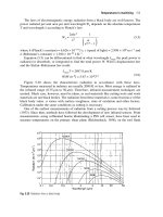
at hand. Figure 1 illustrates the success rates of the five information criteria with re-
Fig. 1. Success rates with minor mixture proportions
spect to minor mixture proportions. Whereas AIC demonstrates a poor performance
across all levels of sample size, CAIC outperforms the other criteria across almost all
factor levels. The criterion performs favorably in recovering the true number of seg-
ments, meeting exemplary chance boundaries for sample sizes of approximately 150
(random chance, proportional chance) and 250 (maximum chance), respectively. The
results in figure 2 from intermediate and near-uniform mixture proportions confirm
the previous findings and underline the CAIC’s strong performance in small sam-
ple size situations, quickly achieving success rates of over 90%. However as sample
sizes increase to 400, both ABIC and AIC3 perform advantageously. Even with near-
unifrom mixture proportions, AIC fails to any meet chance boundaries used in this
set-up. In contrast to previous findings by Andrews and Currim (2003b), CAIC out-
performs BIC across almost all sample/segment size combinations, whereupon the
deviation is marginal in the minor mixture proportion case.
66 Marko Sarstedt and Manfred Schwaiger
Fig. 2. Success rates with intermediate and near-uniform mixture proportions
5 Key contributions and future research directions
The findings presented in this paper are relevant to a large number of researchers
building models using mixture regression analysis. This study extends previous stud-
ies by evaluating how the interaction of sample and segment size affects the perfor-
mance of five of the most widely used information criteria for assessing the true
number of segments in mixture regression models. For the first time the quality of
these criteria was evaluated for a wide spectrum of possible sample/segment-size
constellations. AIC demonstrates an extremely poor performance across all simula-
tion situations. From an application-oriented point of view, this proves to be prob-

Model Selection in Mixture Regression Analysis 67
lematic, taking into account the high percentage of studies relying on this criterion
to assess the number of segments in the model. CAIC performs favourably, show-
ing slight weaknesses in determining the true number of segments for higher sample
sizes, in comparison to ABIC and AIC
3
. Especially in the context of intermediate
and near-uniform mixture proportions AIC
3
performs well, quickly achieving high
success rates.
A continued research on the performance of model selection criteria is needed
in order to provide practical guidelines for disclosing the true number of segments
in a mixture and to guarantee accurate conclusions for marketing practice. In the
present study, only three combinations of mixture proportions were considered, but
as the results show that market characteristics (i.e. different segment sizes) affect
the performance of the criteria, future studies could allow for a greater variation of
these proportions. However, considering the high number of research projects, one
generally has to be critical with the idea of finding a unique measure that can be
considered optimal in every simulation design or even practical applications, as in-
dicated in other studies. Model selection decisions should rather be based on various
evidences, not only derived from the data at hand but also from theoretical consider-
ations.
References
AITKIN, M., RUBIN, D.B. (1985): Estimation and Hypothesis Testing in Finite Mixture Mod-
els. Journal of the Royal Statistical Society, Series B (Methodological), 47 (1), 67-75.
AKAIKE, H. (1973): Information Theory and an Extension of the Maximum Likelihood Prin-
ciple. In B. N. Petrov; F. Csaki (Eds.), Second International Symposium on Information
Theory (267-281). Budapest: Springer.
ANDREWS, R., ANSARI, A., CURRIM, I. (2002): Hierarchical Bayes Versus Finite Mixture

Conjoint Analysis Models: A Comparison of Fit, Prediction and Pathworth Recovery.
Journal of Marketing Research, 39 (1), 87-98.
ANDREWS, R., CURRIM, I. (2003a): A Comparison of Segment Retention Criteria for Finite
Mixture Logit Models. Journal of Marketing Research, 40 (3), 235-243.
ANDREWS, R., CURRIM, I. (2003b): Retention of Latent Segments in Regression-based
Marketing Models. International Journal of Research in Marketing, 20 (4), 315-321.
BOZDOGAN, H. (1987): Model Selection and Akaike’s Information Criterion (AIC): The
General Theory and its Analytical Extensions. Psychometrika, 52 (3), 346-370.
BOZDOGAN, H. (1994): Mixture-model Cluster Analysis using Model Selection Criteria and
a new Information Measure of Complexity. Proceedings of the First US/Japan Confer-
ence on Frontiers of Statistical Modelling: An Informational Approach, Vol. 2 (69-113).
Boston: Kluwer Academic Publishing.
DEMPSTER, A. P., LAIRD, N. M., RUBIN, D. B. (1977): Maximum Likelihood from In-
complete Data via the EM-Algorithm. Journal of the Royal Statistical Society, Series B
(Methodological), 39 (1), 1-39.
DESARBO, W. S., DEGERATU, A., WEDEL, M., SAXTON, M. (2001): The Spatial Repre-
sentation of Market Information. Marketing Science, 20 (4), 426-441.
GRÜN, B., LEISCH, F. (2006): Fitting Mixtures of Generalized Linear Regressions in R.
Computational Statistics and Data Analysis, in press.
68 Marko Sarstedt and Manfred Schwaiger
HAHN, C., JOHNSON, M. D., HERRMANN, A., HUBER, F. (2002): Capturing Customer
Heterogeneity using a Finite Mixture PLS Approach. Schmalenbach Business Review,54
(3), 243-269.
HAWKINS, D. S., ALLEN, D. M., STROMBERG, A. J. (2001): Determining the Number of
Components in Mixtures of Linear Models. Computational Statistics & Data Analysis,
38 (1), 15-48.
JEDIDI, K., JAGPAL, H. S., DESARBO, W. S. (1979): Finite-Mixture Structural Equation
Models for Response-Based Segmentation and Unobserved Heterogeneity. Marketing
Science, 16 (1), 39-59.
LEISCH, F. (2004): FlexMix: A General Framework for Finite Mixture Models and Latent

Class Regresion in R. Journal of Statistical Software, 11 (8), 1-18.
MANTRALA, M. K., SEETHARAMAN, P. B., KAUL, R., GOPALAKRISHNA, S., STAM,
A. (2006): Optimal Pricing Strategies for an Automotive Aftermarket Retailer. Journal
of Marketing Research, 43 (4), 588-604.
MCLACHLAN, G. J., PEEL, D. (2000): Finite Mixture Models, New York: Wiley.
MORRISON, D. G. (1969): On the Interpretation of Discriminant Analysis, Journal of Mar-
keting Research, Vol. 6, 156-163.
OLIVEIRA-BROCHADO, A., MARTINS, F. V. (2006): Examining the Segment Re-
tention Problem for the "Group Satellite" Case. FEP Working Papers, 220.
www.fep.up.pt/investigacao/workingpapers/06.07.04_WP220_brochadomartins
.pdf
RISSANEN, J. (1978): Modelling by Shortest Data Description. Automatica, 14, 465-471.
SARSTEDT, M. (2006): Sample- and Segment-size specific Model Selection in Mix-
ture Regression Analysis. Münchener Wirtschaftswissenschaftliche Beiträge, 08-
2006. Available electronically from />01/2006_08_LMU_sarstedt.pdf
SCHWARZ, G. (1978): Estimating the Dimensions of a Model. The Annals of Statistics, 6 (2),
461-464.
WEDEL, M., KAMAKURA, W. A. (1999): Market Segmentation. Conceptual and Method-
ological Foundations (2nd ed.), Boston, Dordrecht & London: Kluwer.
An Artificial Life Approach
for Semi-supervised Learning
Lutz Herrmann and Alfred Ultsch
Databionics Research Group, Philipps-University Marburg, Germany
{lherrmann,ultsch}@informatik.uni-marburg.de
Abstract. An approach for the integration of supervising information into unsupervised clus-
tering is presented (semi supervised learning). The underlying unsupervised clustering al-
gorithm is based on swarm technologies from the field of Artificial Life systems. Its basic
elements are autonomous agents called Databots. Their unsupervised movement patterns cor-
respond to structural features of a high dimensional data set. Supervising information can be
easily incorporated in such a system through the implementation of special movement strate-

gies. These strategies realize given constraints or cluster information. The system has been
tested on fundamental clustering problems. It outperforms constrained k-means.
1 Introduction
For traditional cluster analysis there is usally a large supply of unlabeled data but
little background information about classes. To generate a complete labeling of
data can be expensive. Instead, background information might be available as small
amount of preclassified input samples that can help to guide the cluster analysis. Con-
sequently, integration of background information into clustering and classification
techniques has recently become focus of interest. See Zhu (2006) for an overview.
Retrieval of previously unknown cluster structures, in the sense of multi-mode
densities, from unclassified and classified data is called semi-supervised clustering.
In contrast to semi-supervised classification, semi-supervised clustering methods are
not limited to the class labels given in the preclassified input samples. New classes
might be discovered, given classes are merged or might be purged.
A particularly promising approach to unsupervised cluster analysis are systems
that possess the ability of emergence through self-organization (Ultsch (2007)). This
means that systems consisting of a huge number of interacting entities may pro-
duce a new, observable pattern on a higher level. Such patterns are said to emerge
from the self-organizing entities. A biological example for emergence through self-
organization is the formation of swarms, e.g. bee swarms or ant colonies.
An example of such nature-inspired information processing techniques is clus-
tering with simulated ants. The ACLUSTER system of Ramos and Abraham (2003)
140 Lutz Herrmann and Alfred Ultsch
is inspired by ant colonies clustering corpses. It consists of a low-dimensional grid
that only carries pheromone intensities. A set of simulated ants moves on the grid’s
nodes. The ants are used to cluster data objects that are located on the grid. An ant
might pick up a data object and drop it later on. Ants are more likely to drop an
object on a node whose neighbourhood has similar data objects rather than on nodes
with dissimilar objects. Ants move according to pheromone trails on the grid.
In this paper we describe a novel approach for semi-supervised clustering that

is based on our unsupervised learning artificial life system (see Ultsch (2000)). The
main idea is that a large number of autonomous agents show collective behaviour
patterns that correspond to structural features of a high dimensional training set. This
approach turns out to be inherently prepared to incorporate additional information
from partially labeled data.
2 Artificial life
The artifical life system (ALife) is used to cluster a finite high-dimensional training
set X ⊂ R
n
. It consists of a low-dimensional grid I ⊂ N
2
and a set B of so-called
Databots. A Databot carries an input sample of training set X and moves on the
grid. Formally, a Databot i ∈ B is denoted as a triple (x
i
,m(x
i
),S
i
) whereas x
i
∈
X is the input sample, m(x
i
) ∈ I is the Databot’s location on the grid and S
i
is a
set of movement programs, so-called strategies. Later on, mapping of data onto the
low-dimensional grid is used for visualization of distance and density structure as
described in section 4.

A strategy s ∈ S
i
is a function that assigns probabilites to available directions
of movement (north, east, et cetera). The Databot’s new location m

(x
i
) is chosen at
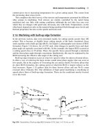
Fig. 1. ALife system: Databots carry high-dimensional data objects while moving on the grid,
nearby objects are to be mapped on nearby nodes of the low-dimensional grid
An Artificial Life Approach for Semi-supervised Learning 141
random according to the strategies’ probabilites. Several strategies are combined into
a single one by weighted averaging of probabilities. Probabilities of movements are
to be chosen such that a Databot is more likely to move towards Databots carrying
similar input samples than towards Databots with dissimilar input samples. This aims
at creation of a sufficiently topography preserving projection m : X → I (see figure
1). For an overview on strategies see Ultsch (2000).
A generalized view on strategies for topography preservation is given below. For
each Databot (x
i
,m(x
i
),S
i
) ∈ B there is a set of bots F
i
(friends) it should move
towards. Here, the strategy for topography preservation is denoted with s
F
. Canoni-

cally, F
i
is chosen to be the Databots carrying the k ∈N most similar input samples
with respect to x
i
according to a given dissimilarity measure d : X ×X → R
+
0
,e.g.
the euclidean metric on cardinal scaled spaces. Strategy s
F
assigns probabilites to
all directions of movements such that m(x
i
) is more likely to be moved towards
1
|F
i
|

j∈F
i
m(x
j
) than to any other node on the grid. This can easily be achieved, for
example, by vectorial addition of distances for every direction of movement. Addi-
tionally, a set of Databots F

i
with the most dissimilar input samples with respect to

x
i
might inversely be used such that m(x
i
) is moved away from its foes. A showclass
example for s
F
is given in figure 2. In analogy to self-organizing maps (Kohonen
(1982)), the size of set F
i
is decreasing over time. This means that Databots adapt a
global ordering before they adapt to local orderings.
Strategies are combined by weighted averaging, i.e. probability of movement towards
direction D ∈{north,east, } is p(D)=

s∈S
i
w
s
s(D)/

s∈S
i
w
s
with w
s
∈ [0,1]
being the weight of strategy s. Linear combination of probabilities is to be preferred
over multiplicative because of its compensation. Several combinations of strategies

have intensely been tested. It turned out that for obtaining good results a small
Fig. 2. Strategies for Databots’ movements: (a) probabilities for directed movements (b) set
of friends (black) and foes (white), counters resulting from vectorial addition of distances are
later on normalized to obtain probabilities, e.g. p
N
consists of black northern distances and
white southern distances
142 Lutz Herrmann and Alfred Ultsch
amount
1
of random walk is necessary. This strategy assigns equal probabilities to
all available directions in order to overcome local optima by the help of randomness.
3 Semi-supervised artificial life
As described in section 2, the ALife system produces a vector projection for clus-
tering purposes using a movement strategy s
F
depending on set F
i
. Choice of bots
in F
i
⊂ B is derived from the input samples’ similarities with respect to x
i
.Thisis
subsumed as unsupervised constraints because F
i
arises from unlabeled data only.
Background information about cluster memberships is given as pairwise con-
straints stating that two input samples x
i

,x
j
∈X belong to the same class (must-link)
or different classes (cannot-link). For each input sample x
i
this results in two sets:
ML
i
⊂ X denotes the samples that are known to belong to the same class whereas
CL
i
⊂ X contains all samples from different classes. ML
i
and CL
i
remain empty for
unclassified input samples. For each x
i
, vector projection m : X → I has to reflect
this by mapping m(x
i
) nearby m(ML
i
) and far from m(CL
i
). This is subsumed as
supervised constraints because they arise from preclassifications.
The s
F
paradigm for satisfaction of unsupervised constraints and how to combine

them has already been described in section 2. Same method is applied for satisfaction
of supervised constraints. This means that an additional strategy s
ML
is introduced
for Databots carrying preclassified input samples. For such a Databot (x
i
,m(x
i
),S
i
)
the set of friends is simply defined as F
i
= ML
i
. According to that strategy, m(x
i
) is
more likely to be moved towards
1
|ML
i
|

j∈ML
i
m(x
j
) than to any other node on the
grid. This strategy s

ML
is added to other available strategies. Thus, integration of su-
pervised and unsupervised learning tasks is realized on basis of movement strategies
for Databots creating a vector projection m.Thisisreferredtoassemi-supervised
learning Databots. The whole system is referred to as semi-supervised ALife (ssAL-
ife).
There are at least two strategies that have to be combined for suitable move-
ment control of semi-supervised learning Databots: the s
F
strategy concerning un-
supervised constraints and the s
ML
strategy concerning supervised constraints. An
adequate proportional weighting of s
F
and s
ML
strategy can be estimated by several
methods: Any clustering method can be understood as a classifier whose quality is
assessable as prediction accuracy. In this case, accuracy means accordance of input
samples’ preclassifications and final clustering. The suitability of a given propor-
tional weighting may be evaluated by cross validation methods. Another approach
is based on two assumptions. First, cluster memberships are rather global than local
qualities. Second, the ssALife system adapts to global orderings before local ones.
Therefore, the influence of the s
ML
strategy is constantly decreasing from 100%
down to 0 over the training process. The latter method was applied in the current
realization of the ssALife system.
1

usually with an absolute weight of 5% up to 10%
An Artificial Life Approach for Semi-supervised Learning 143
4 Semi-Supervised artificial life for cluster analysis
Since ssALife is not an inherent clustering but vector projection method, its visual-
ization capabilities are enhanced using structure maps and the U-Matrix method.
A structure map enhances the regular grid of the ALife system such that each
node i ∈ I contains a high-dimensional codebook vector m
i
∈ R
n
. Structure maps
are used for vector projection and quantization purposes, i.e. arbitrary input sam-
ples x ∈ R
n
are assigned to nodes with bestmatching codebook vectors bm(x)=
argmin
i∈I
d(x, m
i
) with d being the dissimilarity measure from section 2. For a mean-
ingful projection the codebook vectors are to be arranged in a topography preserving
manner. This means that neighbouring nodes i, j usually have got codebook vectors
m
i
,m
j
that are neighbouring in the input space. A popular method to achieve that
is the Emergent Self-organizing Map (see Ultsch (2003)). In this context, projected
input samples m(x
i

),∀x
i
∈X from our ssALife system are used for structure map cre-
ation. A high-dimensional interpolation based on the self-organizing map’s learning
technique determines the codebook vectors (Kohonen (1982)).
The U-Matrix (see figure 3 for illustration) is the canonical display of structure
maps. The local distance structure is displayed on each grid node as a height value
creating a 3D landscape of the high dimensional data space. Clusters are represented
as valleys whereas mountain ranges depict cluster boundaries. See Ultsch (2003) for
an overview.
Contrairy to common belief, visualizations of structure maps are not clustering
algorithms. Segmentation of U-Matrix landscapes into clusters has to be done sepa-
rately. The U*C clustering algorithm uses an entropy-based heuristic in order to au-
tomatically determine the correct number of clusters (Ultsch and Herrmann (2006)).
By the help of the watershed-transformation, a structure map decomposes into sev-
eral coherent regions called basins. Basins are merged in order to form clusters if
they share a highly dense region on the structure map. Therefore, U*C combines
distance and density information for cluster analysis.
5 Experimental settings and results
In order to evaluate the clustering and self-organizing abilities of ssALife, its clus-
tering performance was measured. The main idea is to use data sets on which the
input samples’ true classification is known in beforehand. Clustering accuracy can
be evaluated as fraction of correctly classified input samples. The ssALife is tested
against the well known constrained k-means (COPK-Means) from Wagstaff et al.
(2001). For each data set, both algorithms got 10% of input samples with the true
classification. The remaining samples are presented as unlabeled data.
The data comes from the fundamental clustering problem suite (FCPS). This
is a collection of data sets for testing clustering algorithms. Each data set repre-
sents a certain problem that arbitrary clustering algorithms shall be able to han-
dle when facing real world data sets. For example, ”Chainlink”, ”Atom” and ”Tar-

get” contain spatial clusters of linear not separable, i.e. twined, structure. ”Lsun”,
144 Lutz Herrmann and Alfred Ultsch
”EngyTime” and ”Wingnut” consist of density defined clusters. For details see
/>.
Comparative results can be seen in table 1. The ssALife method clearly out-
performs COPK-Means. COPK-Means suffers from its inability to recognize more
complex cluster shapes. As an example, the so-called EngyTime data set is shown in
figure 3.
Table 1. Percental clustering accuracy: ssALife outperforms COPK-Means, accuracy esti-
mated on fully classified original data over fifty runs with random initialization
data set COPK-Means ssALife with U*C
Atom 71 100
Chainlink 65.7 100
Hepta 100 100
Lsun 96.4 100
Target 55.2 100
Tetra 100 100
TwoDiamonds 100 100
Wingnut 93.4 100
EngyTime 90 96.3
Fig. 3. Density defined clustering problem EngyTime: (a) partially labeled data (b) ssALife
produced U-Matrix, clearly visible decision boundary, fully labeled data
6 Discussion
In this work we described a first approach of semi-supervised cluster analysis using
autonomous agents called Databots. To our knowledge, this is the first approach that
An Artificial Life Approach for Semi-supervised Learning 145
aims for the realization of semi-supervised learning paradigms on basis of a swarm
clustering algorithm.
The ssALife system and Ramos’ ACLUSTER differ in two ways. First, Databots
can be seen as a bijective mapping of input samples onto locations whereas simu-

lated ants have no permanent connection to the data. This facilitates the integration
of additional data-related features into the swarm entities. Furthermore, there is no
global exchange about topographic information in ACLUSTER, which may lead to
discontinuous projections of clusters, i.e. projection errors.
Most popular approaches for semi-supervised learning can be distinguished in
two groups (Belkin et al. (2006)). The manifold assumption states that input samples
with equal class labels are located on manifolds or subspaces, respectively, of the
input space (Belkin et al. (2006), Bilenko et al. (2004)). Recovery of such manifolds
is accomplished by optimization of an objective function, e.g. for adaption of met-
rics. The cluster assumption states that input samples in the same cluster are likely
to have the same class label (Wagstaff et al. (2001), Bilenko et al. (2004)). Again,
recovery of such clusters is accomplished by optimization of an objective function.
Such objective functions consist of terms for unsupervised cluster retrieval and a
loss term that punishes supervised constraint violations. Obviously, the obtainable
clustering solutions are predetermined by the inherent cluster shape assumption of
the chosen objective function. For example, k-means like clustering algorithms and
Mahalanobis like metric adaptions, too, assume linear separable clusters of spheri-
cal shape and well-behaved density structure. In contrast to that, the ssALife method
comes up with a simple yet powerful learning procedure based on movement pro-
grams for autonomous agents. This enables a unification of supervised and unsu-
pervised learning tasks without the need for a main objective function. Except for
the used dissimilarity measure, the ssALife system does not rely on such objective
functions and reaches maximal accuracy on FCPS.
7 Summary
In this paper, cluster analysis is presented on basis of a vector projection problem. Su-
pervised und unsupervised learning of a suitable projection means to incorporate in-
formation from topography and preclassifications of input samples. In order to solve
this, a very simple yet powerful enhancement of our ALife system was introduced.
So-called Databots move the input samples’ projection points on a grid-shaped out-
put space. Databots’ movements are chosen according to so-called strategies. The

unifying framework for supervised and unsupervised learning is simply based on
defining an additional strategy that can incorporate preclassifications into the self-
organization process.
From this self-organizing process a non-linear display of the data’s spatial struc-
ture emerges. The display is used for automatic cluster analysis. The proposed
method ssALife outperforms a simple yet popular algorithm for semi-supervised
cluster analysis.
146 Lutz Herrmann and Alfred Ultsch
References
BELKIN, M., SINDHWANI, V., NIYOGI, P. (2006): The Geometric Basis of Semi-
Supervised Learning. In: O. Chapelle, B. Scholkopf, and A. Zien (Eds.): Semi-Supervised
Learning. MIT Press, 35-54.
BILENKO, M., BASU, S., MOONEY, R.J. (2004): Integrating Constraints and Metric Learn-
ing in Semi-Supervised Clustering. In: Proc. 21st International Conference on Machine
Learning (ICML 2004). Banff, Canada, 81-88.
KOHONEN, T. (1982): Self-organized formation of topologically correct feature maps. In:
Biological Cybernetics (43). 59-69.
RAMOS, V., ABRAHAM, A. (2003): Swarms on Continuous Data. In: Proc. Congress on
Evolutionary Computation. IEEE Press, Australia, 1370-1375.
ULTSCH, A. (2000): Visualization and Classification with Artificial Life. In: Proceedings
Conf. Int. Fed. of Classification Societies (ifcs). Namur, Belgium.
ULTSCH, A. (2003): Maps for the Visualization of high-dimensional Data Spaces. In: Pro-
ceedings Workshop on Self-Organizing Maps (WSOM 2003). Kyushu, Japan, 225-230.
ULTSCH, A., HERRMANN, L. (2006): Automatic Clustering with U*C. Technical Report,
Dept. of Mathematics and Computer Science, University of Marburg.
ULTSCH, A. (2007): Emergence in Self-Organizing Feature Maps. In: Proc. Workshop on
Self-Organizing Maps (WSOM 2007). Bielefeld, Germany, to appear.
WAGSTAFF, K., CARDIE, C., ROGERS, S., SCHROEDL, S. (2001): Constrained K-means
Clustering with Background Knowledge. In: Proc. 18th International Conf. on Machine
Learning. Morgan Kaufmann, San Francisco, CA, 577-584.

ZHU, X. (2006): Semi-Supervised Learning Literature Survey. Computer Sciences TR 1530.
University of Wisconsin, Madison.
Families of Dendrograms
Patrick Erik Bradley
Institut für Industrielle Bauproduktion,
Englerstr. 7, 76128 Karlsruhe, Germany

Abstract. A conceptual framework for cluster analysis from the viewpoint of p-adic geom-
etry is introduced by describing the space of all dendrograms for n datapoints and relating
it to the moduli space of p-adic Riemannian spheres with punctures using a method recently
applied by Murtagh (2004b). This method embeds a dendrogram as a subtree into the Bruhat-
Tits tree associated to the p-adic numbers, and goes back to Cornelissen et al. (2001) in p-adic
geometry. After explaining the definitions, the concept of classifiers is discussed in the con-
text of moduli spaces, and upper bounds for the number of hidden vertices in dendrograms are
given.
1 Introduction
Dendrograms are ultrametric spaces, and ultrametricity is a pervasive property of
observational data, and by Murtagh (2004a) this offers computational advantages
and a well understood basis for developping data processing tools originating in p-
adic arithmetic. The aim of this article is to show that the foundations can be laid
much deeper by taking into account a natural object in p-adic geometry, namely the
Bruhat-Tits tree. This locally finite, regular tree naturally contains the dendrograms
as subtrees which are uniquely determined by assigning p-adic numbers to data.
Hence, the classification task is conceptionally reduced to finding a suitable p-adic
data encoding. Dragovich and Dragovich (2006) find a 5-adic encoding of DNA-
sequences, and Bradley (2007) shows that strings have natural p-adic encodings.
The geometric approach makes it possible to treat time-dependent data on an
equal footing as data that relate only to one instant of time by providing the concept
of family of dendrograms. Probability distributions on families are then seen as a
convenient way of describing classifiers.

Our illustrative toy data set for this article is given as follows:
Example 1.1 Consider the data set D = {0, 1, 3, 4, 12, 20, 32, 64} given by n = 8
natural numbers. We want to hierarchically classify it with respect to the 2-adic
norm |·|
2
as our distance function, as defined in Section 2.
96 Patrick Erik Bradley
2 A brief introduction to p-adic geometry
Euclidean geometry is modelled on the field R of real numbers which are often rep-
resented as decimals, i.e. expanded in powers of the number 10
−1
:
x =
f

Q=m
a
Q
10
−Q
, a
Q
∈{0, ,9}, m ∈Z.
In this way, R completes the field Q of rational numbers with respect to the absolute
norm |x| =

x, x ≥0
−x, x < 0
. On the other hand, the p-adic norm on Q with
|x|

p
=

p
−Q
p
(x)
, x ≡0
0, x = 0
is defined for x =
a
1
a
2
by the difference Q
p
(x)=Q
p
(a
1
) −Q
p
(a
2
) ∈Z in the multiplic-
ities with which numerator and denominator of x are divisible by the prime number
p: a
i
= p
Q

p
(a
i
)
u
i
,andu
i
not divisible by p, i = 1,2.
The p-adic norm satisfies the ultrametric triangle inequality
|x +y|
p
≤ max{|x|
p
,|y|
p
}.
Completing Q with respect to the p-adic norm yields the field Q
p
of p-adic numbers
which is well known to consist of the power series
x =
f

Q=m
a
Q
p
Q
, a

Q
∈{0, ,p −1}, m ∈Z. (1)
Note, that the p-adic expansion is in increasing powers of p, whereas in the decimal
expansion, it is the powers of 10
−1
which increase arbitrarily. An introduction to
p-adic numbers is e.g. Gouvêa (2003).
Example 2.1 For our toy data set D, we have |0|
2
= 0, |1|
2
= |3|
2
= 1, |4|
2
= |12|
2
=
|20|
2
= 2
−2
, |32|
2
= 2
−5
, |64|
2
= 2
−6

, i.e. |·|
2
is maximally 1 on D. Other examples:
|3/2|
3
= |6/4|
3
= 3
−1
, |20|
5
= 5
−1
, |p
−1
|
p
= |p|
−1
p
= p.
Consider the unit disk D = {x ∈Q
p
||x|
p
≤ 1} = B
1
(0). It consists of the so-
called p-adic integers, and is often denoted as Z
p

when emphasizing its ring struc-
ture, i.e. closedness under addition, subtraction and multiplication. A p-adic number
x lies in an arbitrary closed disk B
p
−r (a)={x ∈Q
p
||x−a|
p
≤ p
−r
}, where r ∈ Z,
if and only if x −a is divisible by p
r
. This condition is equivalent to x and a having
the first r termsincommonintheirp-adic expansions (1). The possible radii are all
integer powers of p, so the disjoint disks B
p
−1
(0),B
p
−1
(1), ,B
p
−1
(p −1) are the
maximal proper subdisks of D, as they correspond to truncating the power series (1)
after the constant term. There is a unique minimal disk in which D is contained prop-
erly, namely B
p
(0)={x ∈Q

p
||x|
p
≤ p}. These observations hold true for arbitrary
Families of Dendrograms 97
p-adic disks, i.e. any disk B
p
−r
(x), x ∈ Q
p
, is partitioned into precisely p maximal
subdisks and lies properly in a unique minimal disk. Therefore, if we define a graph
T
Q
p
whose vertices are the p-adic disks, and edges are given by minimal inclusion,
then every vertex of T
Q
p
has precisely p+ 1 outgoing edges. In other words, T
Q
p
is
a p+ 1-regular tree, and p is the size of the residue field F
p
= Z
p
/pZ
p
.

Definition 2.2 The tree T
Q
p
is called the Bruhat-Tits tree for Q
p
.
Remark 2.3 Definition 2.2 is not the usual way to define T
Q
p
. The problem with
this ad-hoc definition is that it does not allow for any action of the projective linear
group PGL
2
(Q
p
).Adefinition invariant under projective linear transformations can
be found e.g. in Herrlich (1980) or Bradley (2006).
An important observation is that any infinite descending chain
B
1
⊇ B
2
⊇ (2)
of strictly decreasing p-adic disks converges to a unique p-adic number {x}=

n
B
n
.
A chain (2) defines a halfline in the Bruhat-Tits tree T

Q
p
.Halflines differing only
by finitely many vertices are said to be equivalent, and the equivalence classes under
this equivalence relation are called ends. Hence the observation means that the p-adic
numbers correspond to ends of T
Q
p
. There is a unique end B
1
⊆ B
2
⊆ coming
from any strictly increasing sequence of disks. This end corresponds to the point at
infinity in the p-adic projective line P
1
(Q
p
)=Q
p
∪{f}, whence the well known
fact:
Lemma 2.4 The ends of T
Q
p
are in one-to-one correspondance with the Q
p
-rational
points of the p-adic projective line P
1

, i.e. with the elements of P
1
(Q
p
).
From the viewpoint of geometry, it is important to distinguish between the p-adic
projective line P
1
as a p-adic manifold and its set P
1
(Q
p
) of Q
p
-rational points, in the
same way as one distinguishes between the affine real line A
1
as a real manifold and
its rational points A
1
(Q)=Q, for example. One reason for distinguishing between a
space and its points is:
Lemma 2.5 Endowed with the metric topology from |·|
p
, the topological space Q
p
is totally disconnected.
The usual approaches towards defining more useful topologies on p-adic spaces
are by introducing more points. Such an approach is the Berkovich topology, which
we will very briefly describe. More details can be found in Berkovich (1990).

The idea is to allow disks whose radii are arbitrary positive real numbers, not
merely powers of p as before. Any strictly descending chain of such disks gives a
point in the sense of Berkovich. For the p-adic line P
1
this amounts to:
Theorem 2.6 (Berkovich) P
1
is non-empty, compact, hausdorff and arc-wise con-
nected. Every point of P
1
\{f} corresponds to a descending sequence B
1
⊇B
2
⊇
of p-adic disks such that B =

B
n
is one of the following:
98 Patrick Erik Bradley
1. a point x in Q
p
,
2. a closed p-adic disk with radius r ∈|Q
p
|
p
,
3. a closed p-adic disk with radius r /∈|Q

p
|
p
,
4. empty.
Points of types 2. to 4. are called generic, points of type 1. classical. We remark
that Berkovich’s definition of points is technically somewhat different and allows
to define more general p-adic spaces. Finally, the Bruhat-Tits tree T
Q
p
is recovered
inside P
1
:
Theorem 2.7 (Berkovich) T
Q
p
is a retract of P
1
\P
1
(Q
p
), i.e. there is a map P
1
\
P
1
(Q
p

) →T
Q
p
whose restriction to T
Q
p
is the identity map on T
Q
p
.
3 p-adic dendrograms
Q
2
0 1 3 4 12 20 32 64
0 f 0022256
1
0 f 100000
3
01f 00 000
4
200f 3422
12
2003f 322
20
2004 3 f 21
32
5002 2 2 f 5
64
6002 2 1 5 f
Fig. 1. 2-adic valuations for D.

0
1
0
1
0
1
2
0
1
3
0
1
4
0
1
5
0
1
6
0
1
0
64
32
4
20
12 1
3
Fig. 2. 2-adic dendrogram for D∪{f}.
Example 3.1 The 2-adic distances within D are encoded in Figure 1, where

dist(i, j)=2
−Q
2
(i, j)
,ifQ
2
(i, j) is the corresponding entry in Figure 1, using 2
−f
= 0.
Figure 2 is the dendrogram for D using |·|
2
: the distance between disjoint clusters
equals the distances between any of their representatives.
Let X ⊆P
1
(Q
p
) be a finite set. By Lemma 2.4, a point of X can be considered as
an end in T
Q
p
.
Definition 3.2 The smallest subtree D (X) of T
Q
p
whose ends are given by X is
called the p-adic dendrogram for X.
Cornelissen et al. (2001) use p-adic dendrograms for studying p-adic symme-
tries, cf. also Cornelissen and Kato (2005). We will ignore vertices in D(X) from
Families of Dendrograms 99

which precisely two edges emanate. Hence, for example, D({0,1,f}) consists of
a unique vertex v(0,1,f) and three ends. The dendrogram for a set X ⊆ N ∪{f}
containing {0,1,f} is a rooted tree with root v(0, 1, f).
Example 3.3 The 2-adic dendrogram in Figure 2 is nothing but D(X) for X = D ∪
{f} and is in fact inspired by the first dendrogram of Murtagh (2004b). The path
from the top cluster to x
i
yields its binary representation [·]
2
which easily translates
into the 2-adic expansion: 0 =[0000000]
2
, 64 =[1000000]
2
= 2
6
, 32 =[0100000]
2
=
2
5
, 4 =[0000100]
2
= 2
2
, 20 =[0010100]
2
= 2
2
+ 2

4
, 12 =[0001100]
2
= 2
2
+ 2
3
,
1 =[0000001]
2
, 3 =[0000011]
2
= 1+ 2
1
.
Any encoding of some data set M which assigns to each x ∈ M a p-adic repre-
sentation of an integer including 0 and 1, yields a p-adic dendrogram D(M ∪{f})
whose root is v(0,1,f), and any dendrogram for real data can be embedded in a non-
unique way into T
Q
p
as a p-adic dendrogram in such a way that v(0,1,f) represents
the top cluster, if p is large enough. In particular, any binary dendrogram is a 2-adic
dendrogram. However, a little algebra helps to find sufficiently large 2-adic Bruhat-
Tits trees T
K
which allow embeddings of arbitrary dendrograms into T
K
. In fact, by
K we mean a finite extension field of Q

p
.Thep-adic norm |·|
p
extends uniquely to a
norm |·|
K
on K, for which it is a complete field, called a p-adic number field.Thein-
tegers of K are again the unit disk
O
K
= {x ∈ K ||x|
K
≤ 1}, and the role of the prime
p is played by a so-called uniformiser S ∈
O
K
. It has the property that O
K
/SO
K
is a
finite field with q = p
f
elements and contains F
p
. Hence, if some dendrogram has a
vertex with maximally n ≥2 children, then we need K large enough such that 2
f
≥n.
This is possible by the results of number theory. Restricting to the prime character-

istic 2 has not only the advantage of avoiding the need to switch the prime number p
in the case of more than p children vertices, but also the arithmetic in 2-adic number
fields is known to be computationally simpler, especially as in our case the so-called
unramified extensions, i.e. where dim
Q
2
K = f ,aresufficient.
Example 3.4 According to Bradley (2007), strings over a finite alphabet can be
encoded in an unramified extension of Q
p
, and hence be classified p-adically.
4 The space of dendrograms
From now on, we will formulate everything for the case K = Q
p
, bearing in mind
that all results hold true for general p-adic number fields K.LetS = {x
1
, ,x
n
}⊆
P
1
(Q
p
) consist of n distinct classical points of P
1
such that x
1
= 0, x
2

= 1, x
3
= f.
Similarly as in Theorem 2.7, the p-adic dendrogram D (S) is a retract of the marked
projective line X = P
1
\S. We call D (S) the skeleton of X. The space of all projective
lines with n such markings is denoted by M
n
, and the space of corresponding p-adic
dendrograms by D
n−1
. M
n
is a p-adic space of dimension n −3, its skeleton D
n−1
is a cw-complex of real polyhedra whose cells of maximal dimension n −3 consist
of the binary dendrograms. Neighbouring cells are passed through by contracting
bounded edges as the n −3 “free” markings “move” about P
1
without colliding. For
100 Patrick Erik Bradley
example, M
3
is just a point corresponding to P
1
\{0,1,f}. M
4
has one free marking
O which can be any Q

p
-rational point from P
1
\{0,1,f}. Hence, the skeleton D
3
is
f
A:
•



>
>
>
>
>
•
z
z
>
>
0
1
O
f
B:
•
~
~

~
>
>
>
>
>
•
z
z
>
>
0
O
1
f
C:
•



>
>
>
>
>
•
y
y
>
>

1
O
0
f
v:
•
{
{
{
{
{
?
?
?
?
?
0
1
O
Fig. 3. Dendrograms representing the different regions of D
3
.
itself a binary dendrogram with precisely one vertex v and three unbounded edges
A,B,C (cf. Figure 3). For n ≥ 3 there are maps
f
n+1
: M
n+1
→ M
n

, I
n+1
: D
n
→ D
n−1
,
which forget the (n + 1)-st marking. Consider a Q
p
-rational point x ∈ M
n
, corre-
sponding to P
1
\S with skeleton d.Itsfibre f
−1
n+1
(x) corresponds to P
1
\S

for all
possible S

whose first n entries constitute S. Hence, the extra marking O ∈ S

\S can
be taken arbitrarily from P(Q
p
) \S. In this way, the space f

−1
n+1
(x) can be considered
as P
1
\S,andI
−1
n+1
(d) as the p-adic dendrogram for S. What we have seen is that tak-
ing fibres recovers the dendrograms corresponding to points in the space D
n
. Instead
of fibres of points, one can take fibres of arbitrary subspaces:
Definition 4.1 A family of dendrograms with n data points over a space Y is a map
Y → D
n
from some p-adic space Y to D
n
.
For example, take Y = {y
1
, ,y
T
}. Then a family Y → D
n
is a time series of
n collision-free particles, if t ∈{1, ,T} is interpreted as time variable. It is also
possible to take into account colliding particles by using compactifications of M
n
as

described in Bradley (2006).
5 Distributions on dendrograms
Given a dendrogram D for some data S = {x
1
, ,x
n
}, the idea of a classifier is
to incorporate a further datum x /∈ S into the classification scheme represented by
D. Often this is done by assigning probabilities to the vertices of D , depending
on x. The result is then a family of possible dendrograms for S ∪{x} with a certain
probability distribution. It is clear that, in the case of p-adic dendrograms, this family
is nothing but I
−1
n+1
(d) →D
n
,ifd ∈D
n−1
is the point representing D . This motivates
the following definition:
Definition 5.1 A universal p-adic classifier
C for n given points is a probability
distribution on M
n+1
.
Families of Dendrograms 101
Here, we take on M
n+1
the Borel V-algebra associated to the open sets of the
Berkovich topology. If x ∈M

n
corresponds to P
1
\S, then C induces a distribution on
f
−1
n+1
(x), hence (after renormalisation) a probability distribution on I
−1
n+1
(d), where
d ∈D
n−1
is the point corresponding to the dendrogram D(S). The similar holds true
for general families of dendrograms, e.g. time series of particles.
6 Hidden vertices
A vertex v in a p-adic dendrogram D is called hidden, if the class corresponding
to v is not the top class and does not directly contain data points but is composed
of non-trivial subclasses. The subforest of D spanned by its hidden vertices will be
denoted by D
h
, and is called the hidden part of D. The number b
h
0
of connected
components of D
h
measures how the clusters corresponding to non-hidden vertices
are spread within the dendrogram D . We give bounds for b
h

0
and the number v
h
of
hidden vertices, and refer to Bradley (2006) for the combinatorial proofs (Theorems
8.3 and 8.5).
Theorem 6.1 Let D ∈D
n
.Then
v
h
≤
n +2−b
h
0
2
and b
h
0
≤
n −4
3
,
where the latter bound is sharp.
7 Conclusions
Since ultrametricity is the natural property which allows classification and is perva-
sive in observational data, the techniques of ultrametric analysis and p-adic geometry
are at ones disposal for identifying and exploiting ultrametricity. A p-adic encoding
of data provides a way to investigate arithmetic properties of the p-adic numbers
representing the data.

It is our aim to lay the geometric foundation towards p-adic data encoding. From
the geometric point of view it is natural to perform the encoding by embedding its
underlying dendrogram into the Bruhat-Tits tree. In fact, the dendrogram and its em-
bedding are uniquely determined by the p-adic numbers representing the data. For
this end, we give an account of p-adic geometry in order to define p-adic dendro-
grams as subtrees of the Bruhat-Tits tree.
In the next step we introduce the space of all dendrograms for a given num-
ber of data points which, by p-adic geometry, is contained in the space M
n
of all
marked projective lines, an object appearing in the context of the classification of
Riemann surfaces. The advantages of considering the space of dendrograms rely on
the fact that a conceptual formulation of moving particles as families of dendrograms
is made possible, and its simple geometry as a polyhedral complex. Also, assigning
distributions on M
n
allows for probabilistic incorporation of further data to a given
102 Patrick Erik Bradley
dendrogram. At the end, we give bounds for the numbers of hidden vertices and
hidden components of dendrograms.
What remains to do is to computationally exploit the foundations laid in this
article by developping a code along these lines and apply it to Fionn Murtagh’s task
of finding ultrametricity in data.
Acknowledgements
The author is supported by the Deutsche Forschungsgemeinschaft through the re-
search project Dynamische Gebäudebestandsklassifikation BR 3513/1-1, and thanks
Hans-Hermann Bock for suggesting to include a toy dataset, and an unknown referee
for many valuable remarks.
References
BERKOVICH, V.G. (1990): Spectral Theory and Analytic Geometry over Non-Archimedean

Fields. Mathematical Surveys and Monographs, 33, AMS.
BRADLEY, P.E. (2006): Degenerating families of dendrograms. Preprint.
BRADLEY, P.E. (2007): Mumford dendrograms. Preprint.
CORNELISSEN, G. and KATO, F. (2005): The p-adic icosahedron. Notices of the AMS, 52,
720–727.
CORNELISSEN, G., KATO, F. and KONTOGEORGIS, A. (2001): Discontinuous groups in
positive characteristic and automorphisms of Mumford curves. Mathematische Annalen,
320, 55–85.
DRAGOVICH, B. AND DRAGOVICH, A. (2006): A p-Adic Model of DNA-Sequence and
Genetic Code. Preprint
arXiv:q-bio.GN/0607018
.
GOUVÊA, F.Q. (2003): p-adic numbers: an introduction. Universitext, Springer.
HERRLICH, F (1980): Endlich erzeugbare p-adische diskontinuierliche Gruppen. Archiv der
Mathematik, 35, 505–515.
MURTAGH, F. (2004): On ultrametricity, data coding, and computation. Journal of Classifi-
cation, 21, 167–184.
MURTAGH, F. (2004): Thinking ultrametrically. In: D. Banks, L. House, F.R. McMorris, P.
Arabie, and W. Gaul (Eds.): Classification, Clustering and Data Mining, Springer, 3–14.
Hard and Soft Euclidean Consensus Partitions
Kurt Hornik and Walter Böhm
Department of Statistics and Mathematics
Wirtschaftsuniversität Wien, A-1090 Wien, Austria
{Kurt.Hornik, Walter.Boehm}@wu-wien.ac.at
Abstract. Euclidean partition dissimilarity d(P,
˜
P) (Dimitriadou et al., 2002) is defined as the
square root of the minimal sum of squared differences of the class membership values of the
partitions P and
˜

P, with the minimum taken over all matchings between the classes of the parti-
tions. We first discuss some theoretical properties of this dissimilarity measure. Then, we look
at the Euclidean consensus problem for partition ensembles, i.e., the problem to find a hard
or soft partition P with a given number of classes which minimizes the (possibly weighted)
sum

b
w
b
d(P
b
,P)
2
of squared Euclidean dissimilarities d between P and the elements P
b
of the ensemble. This is an NP-hard problem, and related to consensus problems studied in
Gordon and Vichi (2001). We present an efficient “Alternating Optimization” (AO) heuristic
for finding P, which iterates between optimally rematching classes for fixed memberships, and
optimizing class memberships for fixed matchings. An implementation of such AO algorithms
for consensus partitions is available in the R extension package clue. We illustrate this algo-
rithm on two data sets (the popular Rosenberg-Kim kinship terms data and a macroeconomic
one) employed by Gordon & Vichi.
1 Introduction
Over the years, a huge number of dissimilarity measures for (hard) partitions has
been suggested. Day (1981), building on work by Boorman and Arabie (1972), iden-
tifies two leading groups of such measures. Supervaluation metrics are derived from
supervaluations on the lattice of partitions. Minimum cost flow (MCF) metrics are
given by the minimum weighted number of admissible transformations required to
transform one partition into another.
One such MCF metric is the R-metric of Rubin (1967), defined as the “mini-

mal number of augmentations and removals of single objects” needed to transform
one partition into another. This equals twice the Boorman-Arabie A (single element
moves) distance, and is also called transfer distance in Charon et al. (2006) and
partition-distance in Gusfield (2002). It can be computed by solving the Linear Sum
Assignment Problem (LSAP)
min
W∈W
A

k,l
w
kl
|C
k
'
˜
C
l
|
148 Kurt Hornik and Walter Böhm
where W
A
is the set of all matrices W =[w
kl
] with non-negative elements and row all
column sums all one, and the {C
k
}and {
˜
C

l
}denote the classes of the first and second
partition P and
˜
P, respectively. The LSAP can be solved efficiently in polynomial
time using primal-dual algorithms such as the so-called Hungarian method, see e.g.
Papadimitriou and Steiglitz (1982).
For possibly soft partitions, as e.g. obtained by fuzzy or model-based mixture
clustering, the theory of dissimilarities is far less developed. To fix notations and ter-
minology, let n be the number of objects to be classified. A (possibly soft) partition P
assigns to each object i and class k a non-negative number m
ik
quantifying the “be-
longingness” or membership of the object to the class, such that

k
m
ik
= 1. We can
gather the m
ik
into the membership (matrix) M = M(P)=[m
ik
] of the partition. In
general, M is a stochastic matrix; for hard partitions, it is a binary matrix. Note that
M is unique up to permutations of its columns. We refer to the number of non-zero
columns of M as the number of classes of the partition, and write
P
Q
and P

H
Q
for the
space of all (possibly soft) partitions with Q classes, and all hard partitions with Q
classes, respectively.
In what follows, it will often be convenient to bring memberships to “a com-
mon number of classes” (i.e., columns) by adding trailing zero columns as needed.
Formally, we can work on the space
P of all stochastic matrices with n rows and in-
finitely many columns, with the normalization that non-zero columns are the leading
ones.
For two hard partitions with memberships M and
˜
M,wehave|C
k
'
˜
C
l
| =

i
|m
ik
− ˜m
il
|
p
for all p ≥ 1, as |u|
p

= |u| if u ∈{−1,0,1}. This strongly suggests
to generalize the R-metric to possibly soft partitions via dissimilarities defined as the
p-th root of
min
W∈W
A

k,l
w
kl

i
|m
ik
− ˜m
il
|
p
Using p = 2givesEuclidean dissimilarity d (Dimitriadou et al. (2002)). Identify-
ing the optimal assignment with its corresponding map S (“permutation” in the pos-
sibly augmented case) of the classes of the first to those of the second partition (i.e.,
S(k)=l iff w
kl
= 1iffC
k
is matched with
˜
C
l
), we can use


k,l
w
kl

i
|m
ik
− ˜m
il
|
p
=

i

k
|m
ik
− ˜m
i,S(k)
|
p
to obtain
d(M,
˜
M)=min
3
M −
˜

M3
F
where the minimum is taken over all permutation matrices 3 and M
F
=
(

i,k
m
2
ik
)
1/2
is the Frobenius norm. See Hornik (2005b) for details.
For p = 1, we get Manhattan dissimilarity (Hornik, 2005a). For general p and
W =[w
kl
] constrained to have given row sums D
k
and column sums E
l
(not neces-
sarily all identical as for the assignment case), we get the Mallows-type distances
introduced in Zhou et al. (2005), and motivated from formulations of the Monge-
Kantorovich optimal mass transfer problem.
Gordon and Vichi (2001, Model 1) introduce a dissimilarity measure also based
on squared distances between optimally matched columns of the membership matri-
ces, but ignoring the “unmatched” columns. This will result in discontinuities (with
Hard and Soft Euclidean Consensus Partitions 149
respect to the natural topology on P ) for sequences of membership matrices for

which at least one column converges to zero.
In Section 2, we give some theoretical results related to Euclidean partition dis-
similarity, and present a heuristic for solving the Euclidean consensus problem for
partition ensembles. Section 3 investigates soft Euclidean consensus partitions for
two data sets employed in Gordon and Vichi (2001), the popular Rosenberg-Kim
kinship terms data and a macroeconomic one.
2 Theory
2.1 Maximal Euclidean dissimilarity
Charon et al. (2006) provide closed-form expressions for the maximal R-metric
(transfer distance) between hard partitions with Q and
˜
Q classes, which readily yield
z
Q,
˜
Q
= max
M∈P
H
Q
,
˜
M∈P
H
˜
Q
d(M,
˜
M)=


n −c
min
(Q,
˜
Q),
with the minimum concordance c
min
given in Theorem 2 of Charon et al. (2006). One
can show (Hornik, 2007b) that the maxima of the Euclidean dissimilarity between
(possibly soft) partitions can always be attained at the “boundary”, i.e., for hard
partitions, such that
max
M∈P
Q
,
˜
M∈P
˜
Q
d(M,
˜
M)= max
M∈P
H
Q
,
˜
M∈P
H
˜

Q
d(M,
˜
M)=z
Q,
˜
Q
E.g., if Q ≤
˜
Q and (Q −1)
˜
Q < n,thenz
Q,
˜
Q
=(n−n/
˜
Q)
1/2
. Note that the dissimilar-
ities between soft partitions are “typically” much smaller than for hard ones.
2.2 The Euclidean consensus problem
Aggregating ensembles of clusterings into a consensus clustering by minimiz-
ing average dissimilarity has a long history, with key contributions including
Mirkin (1974), Barthélemy and Monjardet (1981, 1988), and Wakabayashi (1998).
More generally, clusterwise aggregation of ensembles of relations (thus containing
equivalence relations, i.e., partitions, as a special case) was introduced by Gaul and
Schader (1988).
Given an ensemble (profile) of partitions P
1

, ,P
B
of the same n objects and
weights w
1
, ,w
B
summing to one, a soft Euclidean consensus partition (general-
ized mean partition) is defined as a partition which minimizes

B
b=1
w
b
d(P,P
b
)
2
over P
Q
for given Q. Similarly, a hard Euclidean consensus partition minimizes the
criterion function over
P
H
Q
. Equivalently, one needs to find
150 Kurt Hornik and Walter Böhm
min
M


b
w
b
min
3
b
M −M
b
3
b

2
F
= min
M
min
3
1
, ,3
b

b
w
b
M −M
b
3
b

2

F
over all suitable M and permutation matrices 3
1
, ,3
B
.
Soft Euclidean consensus partitions can be characterized as follows (see
Hornik (2005b)). For fixed 3
1
, ,3
B
,

b
w
b
M − M
b
3
b

2
F
= M −
¯
M
2
F
+


b
w
b
M
b
3
b

2
F
−
¯
M
2
F
where
¯
M =

b
w
b
M
b
3
b
is the weighted mean of the (suit-
ably matched) memberships. If
¯
M is feasible for M (such that Q ≥max(Q

1
, ,Q
B
)),
the overall minimum sought is found by
max
3
1
, ,3
B

¯
M
2
F
= max
3
1
, ,3
B

Q
k=1
c
S
1
(k), ,S
B
(k)
,

for a suitable B-dimensional cost array c. This is an instance of the Multi-dimensional
Assignment Problem (MAP), which is known to be NP-hard.
For hard partitions M and fixed 3
1
, ,3
B
,

b
w
b
M − M
b
3
b

2
F
=
M
2
F
− 2

b
w
b
trace(M

M

b
3
b
)+

b
w
b
M
b
3
b

2
F
= const − 2trace(M

¯
M). As
trace(M

¯
M)=

i

k
m
ik
¯m

ik
,ifagainQ ≥ max(Q
1
, ,Q
B
), this can be maximized
by choosing, for each row i, m
ik
= 1forthefirst k such that ¯m
ik
is maximal for the
i-th row of
¯
M. I.e., the optimal M is given by a closest hard partition H(
¯
M) of
¯
M
(“winner-takes-all weighted voting”).
Inserting the optimal M yields that the optimal permutations are found by solving
max
3
1
, ,3
B

i

max
1≤k≤Q


b
w
b
m
i,S
b
(k)

which looks “similar” to, if not worse than, the MAP for the soft case.
In both cases, we find that determining Euclidean consensus partitions by simul-
taneous optimization over the memberships M and permutations 3
1
, ,3
B
leads
to very hard combinatorial optimization problems, for which solutions by exhaus-
tive search are only possible for very “small” instances. Hornik and Böhm (2007)
introduce an “Alternating Optimization” (AO) algorithm based on the natural idea to
alternate between minimizing the criterion function

b
w
b
M −M
b
3
b

2

F
over the
permutation for fixed M, and over M for fixed permutations. The first amounts to
solving B (independent) linear sum assignment problems, the latter to computing
suitable approximations to the weighted mean
¯
M =

b
w
b
M
b
3
b
(see above for the
case where Q ≥ max(Q
1
, ,Q
B
); otherwise, one needs to “project” or constrain to
the space of all M with only Q leading non-zero columns). If every update reduces
the criterion function, converge to a fixed point is ensured (it is currently unknown
whether these are necessarily local minima of the criterion function). These AO al-
gorithms, which are implemented as methods
"SE"
(default) and
"HE"
of function
cl_consensus

of package clue (Hornik, 2007a), provide efficient heuristics for find-
ing the global optimum, provided that the best solution found in “sufficiently many”
replications with random starting values is employed.
Hard and Soft Euclidean Consensus Partitions 151
Table 1. Memberships for the soft Euclidean consensus partition with Q = 3 classes for the
Gordon-Vichi macroeconomic ensemble.
Argentina
0.618 0.374 0.008
Bolivia
0.666 0.056 0.278
Canada 0.018
0.980 0.002
Chile
0.632 0.356 0.012
Egypt
0.750 0.070 0.180
France 0.012
0.988 0.000
Greece
0.736 0.194 0.070
India
0.542 0.076 0.382
Indonesia
0.616 0.144 0.240
Italy 0.044
0.950 0.006
Japan 0.134
0.846 0.020
Norway 0.082
0.912 0.006

Portugal
0.488 0.452 0.060
South Africa
0.626 0.366 0.008
Spain 0.314
0.658 0.028
Sudan
0.566 0.088 0.346
Sweden 0.050
0.944 0.006
U.K. 0.112
0.872 0.016
U.S.A. 0.062
0.930 0.008
Uruguay
0.680 0.310 0.010
Venezuela
0.600 0.390 0.010
3 Applications
3.1 Gordon-Vichi macroeconomic ensemble
Gordon and Vichi (2001, Table 1) provide soft partitions of 21 countries based on
macroeconomic data for the years 1975, 1980, 1985, 1990, and 1995. These parti-
tions were obtained using fuzzy c-means on measurements of variables such as an-
nual per capita gross domestic product (GDP) and the percentage of GDP provided
by agriculture. The 1980 and 1990 partitions have 3 classes, the remaining ones two.
Table 1 shows the memberships of the soft Euclidean consensus partition for
Q = 3 based on 1000 replications of the AO algorithm. It can be verified by exhaus-
tive search (which is feasible as there are at most 6
5
= 7776 possible permutation

sequences) that this is indeed the optimal solution. Interestingly, one can see that
the maximal membership values are never attained in the third column, such that
the corresponding closest hard partition (which is also the hard Euclidean consen-
sus partition) has only 2 classes. One might hypothesize that there is a bias towards
2-class partitions as these form the majority (3 out of 5) of the data set, and that
3-class consensus partitions could be obtained by suitably “up-sampling” the 3-class
partitions, i.e., increasing their weights w
b
. Table 2 indicates how a third consensus
class is formed when giving the 3-class partitions w times the weight of the 2-class
ones (all these countries are in class 1 for the unweighted consensus partition): The
order in which countries join this third class (of the least developed countries) agrees
very well with the “sureness” of their classification in the unweighted consensus, as
measured by their margins, i.e., the difference between the largest and second largest
membership values for the respective objects.
3.2 Rosenberg-Kim Kinship terms data
Rosenberg and Kim (1975) describe an experiment where perceived similarities of
the kinship terms were obtained from six different “sorting” experiments. In one of