Data Analysis Machine Learning and Applications Episode 1 Part 6 docx

152 Kurt Hornik and Walter Böhm
Table 2. Formation of a third class in the Euclidean consensus partitions for the Gordon-Vichi
macroeconomic ensemble as a function of the weight ratio w between 3- and 2-class partitions
in the ensemble.
1.5 India
2.0 India, Sudan
3.0 India, Sudan
4.5 India, Sudan, Bolivia, Indonesia
10.0 India, Sudan, Bolivia, Indonesia
12.5 India, Sudan, Bolivia, Indonesia, Egypt
f India, Sudan, Bolivia, Indonesia, Egypt
these, 85 female undergraduates at Rutgers University were asked to sort 15 English
terms into classes “on the basis of some aspect of meaning”. There are at least three
“axes” for classification: gender, generation, and direct versus indirect lineage. The
Euclidean consensus partitions with Q = 3 classes put grandparents and grandchil-
dren in one class and all indirect kins into another one. For Q = 4, {brother, sister}
are separated from {father, mother, daughter, son}. Table 3 shows the memberships
for a soft Euclidean consensus partition for Q = 5 based on 1000 replications of the
AO algorithm.
Table 3. Memberships for the 5-class soft Euclidean consensus partition for the Rosenberg-
Kim kinship terms data.
grandfather 0.000 0.024 0.012
0.965 0.000
grandmother 0.005 0.134 0.016
0.840 0.005
granddaughter 0.113 0.242 0.054
0.466 0.125
grandson 0.134 0.111 0.052
0.581 0.122
brother
0.612 0.282 0.024 0.082 0.000

sister
0.579 0.391 0.026 0.002 0.002
father 0.099
0.546 0.122 0.158 0.075
mother 0.089
0.654 0.136 0.054 0.066
daughter 0.000
1.000 0.000 0.000 0.000
son 0.031
0.842 0.007 0.113 0.007
nephew 0.012 0.047 0.424 0.071
0.447
niece 0.000 0.129
0.435 0.000 0.435
cousin 0.080 0.056
0.656 0.033 0.174
aunt 0.000 0.071
0.929 0.000 0.000
uncle 0.000 0.000
0.882 0.071 0.047
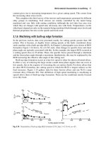
Figure 1 indicates the classes and margins for the 5-class solutions. We see that
the memberships of ‘niece’ are tied between columns 3 and 5, and that the margin
of ‘nephew’ is only very small (0.02), suggesting the 4-class solution as the optimal
Euclidean consensus representation of the ensemble.
Hard and Soft Euclidean Consensus Partitions 153
uncle
aunt
cousin
niece
nephew

son
daughter
mother
father
sister
brother
grandson
granddaughter
grandmother
grandfather
0.0 0.2 0.4 0.6 0.8 1.0
4
4
4
4
1
1
2
2
2
2
5
3/5
3
3
3
Fig. 1. Classes (incicated by plot symbol and class id) and margins (differences between the
largest and second largest membership values) for the 5-class soft Euclidean consensus parti-
tion for the Rosenberg-Kim kinship terms data.
Quite interestingly, none of these consensus partitions split according to gender,

even though there are such partitions in the data. To take the natural heterogene-
ity in the data into account, one could try to partition them (perform clusterwise
aggregation, Gaul and Schader (1988)), resulting in meta-partitions (Gordon and
Vichi (1998)) of the underlying objects. Function
cl_pclust
in package clue pro-
vides an AO heuristic for soft prototype-based partitioning of classifications, allow-
ing in particular to obtain soft or hard meta-partitions with soft or hard Euclidean
consensus partitions as prototypes.
References
BARTHÉLEMY, J.P. and MONJARDET, B. (1981): The median procedure in cluster analysis
and social choice theory. Mathematical Social Sciences, 1, 235–267.
BARTHÉLEMY, J.P. and MONJARDET, B. (1988): The median procedure in data analysis:
new results and open problems. In: H. H. Bock, editor, Classification and related methods
of data analysis. North-Holland, Amsterdam, 309–316.
BOORMAN, S. A. and ARABIE, P. (1972): Structural measures and the method of sorting.
In R. N. Shepard, A. K. Romney and S. B. Nerlove, editors, Multidimensional Scaling:
Theory and Applications in the Behavioral Sciences, 1: Theory. Seminar Press, New
York, 225–249.
CHARON, I., DENOEUD, L., GUENOCHE, A. and HUDRY, O. (2006): Maximum transfer
distance between partitions. Journal of Classification, 23(1), 103–121.
DAY, W. H. E. (1981): The complexity of computing metric distances between partitions.
Mathematical Social Sciences, 1, 269–287.
DIMITRIADOU, E., WEINGESSEL, A. and HORNIK, K. (2002): A combination scheme for
fuzzy clustering. International Journal of Pattern Recognition and Artificial Intelligence,
16(7), 901–912.
GAUL, W. and SCHADER, M. (1988): Clusterwise aggregation of relations. Applied Stochas-
tic Models and Data Analysis, 4, 273–282.
154 Kurt Hornik and Walter Böhm
GORDON, A. D. and VICHI, M. (1998): Partitions of partitions. Journal of Classification,

15, 265–285.
GORDON, A. D. and VICHI, M. (2001): Fuzzy partition models for fitting a set of partitions.
Psychometrika, 66(2), 229–248.
GUSFIELD, D. (2002): Partition-distance: A problem and class of perfect graphs arising in
clustering. Information Processing Letters, 82, 159–164.
HORNIK, K. (2005a): A CLUE for CLUster Ensembles. Journal of Statistical Software,
14(12). URL
/>.
HORNIK, K. (2005b): Cluster ensembles. In C. Weihs and W. Gaul, editors, Classifi-
cation – The Ubiquitous Challenge. Proceedings of the 28th Annual Conference of
the Gesellschaft für Klassifikation e.V., University of Dortmund, March 9–11, 2004.
Springer-Verlag, Heidelberg, 65–72.
HORNIK, K. (2007a): clue: Cluster Ensembles. R package version 0.3-12.
HORNIK, K. (2007b): On maximal euclidean partition dissimilarity. Under preparation.
HORNIK, K. and BÖHM, W. (2007): Alternating optimization algorithms for Euclidean and
Manhattan consensus partitions. Under preparation.
MIRKIN, B.G. (1974): The problem of approximation in space of relations and qualitative
data analysis. Automatika y Telemechanika, translated in: Information and Remote Con-
trol, 35, 1424–1438.
PAPADIMITRIOU, C. and STEIGLITZ, K. (1982): Combinatorial Optimization: Algorithms
and Complexity. Prentice Hall, Englewood Cliffs.
ROSENBERG, S. (1982): The method of sorting in multivariate research with applications
selected from cognitive psychology and person perception. In N. Hirschberg and L. G.
Humphreys, editors, Multivariate Applications in the Social Sciences. Erlbaum, Hills-
dale, New Jersey, 117–142.
ROSENBERG, S. and KIM, M. P. (1975): The method of sorting as a data-gathering procedure
in multivariate research. Multivariate Behavioral Research, 10, 489–502.
RUBIN, J. (1967): Optimal classification into groups: An approach for solving the taxonomy
problem. Journal of Theoretical Biology, 15, 103–144.
WAKABAYASHI, Y. (1998): The complexity of computing median relations. Resenhas do

Instituto de Mathematica ed Estadistica, Universidade de Sao Paolo, 3/3, 323–349.
ZHOU, D., LI, J. and ZHA, H. (2005): A new Mallows distance based metric for comparing
clusterings. In ICML ’05: Proceedings of the 22nd International Conference on Machine
Learning. ISBN 1-59593-180-5. ACM Press, New York, NY, USA, 1028–1035.
Information Integration of Partially
Labeled Data
Steffen Rendle and Lars Schmidt-Thieme
Information Systems and Machine Learning Lab, University of Hildesheim
{srendle, schmidt-thieme}@ismll.uni-hildesheim.de
Abstract. A central task when integrating data from different sources is to detect identical
items. For example, price comparison websites have to identify offers for identical products.
This task is known, among others, as record linkage, object identification, or duplicate detec-
tion.
In this work, we examine problem settings where some relations between items are given
in advance – for example by EAN article codes in an e-commerce scenario or by manually
labeled parts. To represent and solve these problems we bring in ideas of semi-supervised and
constrained clustering in terms of pairwise must-link and cannot-link constraints. We show
that extending object identification by pairwise constraints results in an expressive framework
that subsumes many variants of the integration problem like traditional object identification,
matching, iterative problems or an active learning setting.
For solving these integration tasks, we propose an extension to current object identification
models that assures consistent solutions to problems with constraints. Our evaluation shows
that additionally taking the labeled data into account dramatically increases the quality of
state-of-the-art object identification systems.
1 Introduction
When information collected from many sources should be integrated, different ob-
jects may refer to the same underlying entity. Object identification aims at identifying
such equivalent objects. A typical scenario is a price comparison system where offers
from different shops are collected and identical products have to be found. Decisions
about identities are based on noisy attributes like product names or brands. More-

over, often some parts of the data provide some kind of label that can additionally
be used. For example some offers might be labeled by a European Article Number
(EAN) or an International Standard Book Number (ISBN). In this work we investi-
gate problem settings where such information is provided on some parts of the data.
We will present three different kinds of knowledge that restricts the set of consistent
solutions. For solving these constrained object identification problems we extend the
generic object identification model by a collective decision model that is guided by
both constraints and similarities.
172 Steffen Rendle and Lars Schmidt-Thieme
2 Related work
Object identification (e.g. Neiling 2005) is also known as record linkage (e.g. Win-
kler 1999) and duplicate detection (e.g. Bilenko and Mooney 2003). State-of-the-art
methods use an adaptive approach and learn a similarity measure that is used for
predicting the equivalence relation (e.g. Cohen and Richman 2002). In contrast, our
approach also takes labels in terms of constraints into account.
Using pairwise constraints for guiding decisions is studied in the community of
semi-supervised or constrained clustering – e.g. Basu et al. (2004). However, the
problem setting in object identification differs from this scenario because in semi-
supervised clustering typically a small number of classes is considered and often it is
assumed that the number of classes is known in advance. Moreover, semi-supervised
clustering does not use expensive pairwise models that are common in object identi-
fication.
3 Four problem classes
In the classical object identification problem C
classic
a set of objects X should be
grouped into equivalence classes E
X
. In an adaptive setting, a second set Y of objects
is available where the perfect equivalence relation E

Y
is known. It is assumed that X
and Y are disjoint and share no classes – i.e. E
X
∩E
Y
=

.
In real world problems often there is no such clear separation between labeled
and unlabeled data. Instead only the objects of some subset Y of X are labeled. We
call this problem setting the iterative problem
C
iter
where (X,Y,E
Y
) is given with
X ⊇Y and Y
2
⊇E
Y
. Obviously, consistent solutions E
X
have to satisfy E
X
∩Y
2
= E
Y
.

Examples of applications for iterative problems are the integration of offers from
different sources where some offers are labeled by a unique identifier like an EAN
or ISBN, and iterative integration tasks where an already integrated set of objects is
extended by new objects.
The third problem setting deals with integrating data from n sources, where each
source is assumed to contain no duplicates at all. This is called the class of matching
problems
C
match
. Here the problem is given by X = {X
1
, ,X
n
} with X
i
∩X
j
=


and the set of consistent equivalence relations
E is restricted to relations E on X
with E ∩X
2
i
= {(x, x)|x ∈ X
i
}. Traditional record linkage often deals with matching
problems of two data sets (n = 2).
At last, there is the class of pairwise constrained problems

C
constr
. Here each
problem is defined by (X,R
ml
,R
cl
) where the set of objects X is constrained by a
must-link R
ml
and a cannot-link relation R
cl
. Consistent solutions are restricted to
equivalence releations E with E ∩R
cl
=

 and E ⊇ R
ml
. Obviously, R
cl
is symmet-
ric and irreflexive whereas R
ml
has to be an equivalence relation. In all, pairwise
constrained problems differ from iterative problems by labeling relations instead of
labeling objects. The constrained problem class can better describe local informa-
tions like two offers are the same/ different. Such information can for example be
provided by a human expert in an active learning setting.
Information Integration of Partially Labeled Data 173

Fig. 1. Relations between problem classes: C
classic
⊂ C
iter
⊂ C
constr
and C
classic
⊂ C
match
⊂
C
constr
.
We will show, that the presented problem classes form a hierarchy C
classic
⊂
C
iter
⊂ C
constr
and that C
classic
⊂ C
match
⊂ C
constr
but neither C
match
⊆ C

iter
nor C
iter
⊆
C
match
(see Figure 1). First of all, it is easy to see that C
classic
⊆ C
iter
because any
problem X ∈
C
classic
corresponds to an iterative problem without labeled data (Y =

). Also
C
classic
⊆ C
match
because an arbitrary problem X ∈ C
classic
can be trans-
formed to a matching problem by considering each object as its own dataset: X
1
=
{x
1
}, ,X

n
= {x
n
}. On the other hand, C
iter
⊆ C
classic
and C
match
⊆ C
classic
, because
C
classic
is not able to formulate any restriction on the set of possible solutions E as
the other classes can do. This shows that:
C
classic
⊂ C
match
, C
classic
⊂ C
iter
(1)
Next we will show that
C
iter
⊂C
constr

. First of all, any iterative problem (X,Y, E
Y
)
can be transformed to a constrained problem (X,R
ml
,R
cl
) by setting
R
ml
←{(y
1
,y
2
)|y
1
≡
E
Y
y
2
} and R
cl
←{(y
1
,y
2
)|y
1
≡

E
Y
y
2
}. On the other hand, there
are problems (X,R
ml
,R
cl
) ∈ C
constr
that cannot be expressed as an iterative problem,
e.g.:
X = {x
1
,x
2
,x
3
,x
4
}, R
ml
= {(x
1
,x
2
),(x
3
,x

4
)}, R
cl
=


If one tries to express this as an iterative problem, one would assign to the pair (x
1
,x
2
)
the label l
1
and to (x
3
,x
4
) the label l
2
. But one has to decide whether or not l
1
= l
2
.
If l
1
= l
2
, then the corresponding constrained problem would include the constraint
(x

2
,x
3
) ∈ R
ml
, which differs from the original problem. Otherwise, if l
1
= l
2
,this
would imply (x
2
,x
3
) ∈ R
cl
, which again is a different problem. Therefore:
C
iter
⊂ C
constr
(2)
Furthermore,
C
match
⊆ C
constr
because any matching problem X
1
, ,X

n
can be
expressed as a constrained problem with:
X =
n

i=1
X
i
, R
cl
= {(x,y)|x,y ∈X
i
∧x = y}, R
ml
=


There are constrained problems that cannot be translated into a matching problem.
E.g.:
174 Steffen Rendle and Lars Schmidt-Thieme
X = {x
1
,x
2
,x
3
}, R
ml
= {(x

1
,x
2
)}, R
cl
=


Thus:
C
match
⊂ C
constr
(3)
At last, there are iterative problems that cannot be expressed as matching prob-
lems, e.g.:
X = {x
1
,x
2
,x
3
}, Y = {x
1
,x
2
}, x
1
≡
E

Y
x
2
And there are matching problems that have no corresponding iterative problem, e.g.:
X
1
= {x
1
,x
2
}, X
2
= {y
1
,y
2
}
Therefore:
C
match
⊆ C
iter
, C
iter
⊆ C
match
(4)
In all we have shown that
C
constr

is the most expressive class and subsumes all
the other classes.
4 Method
Object Identification is generally done by three core components (Rendle and Schmidt-
Thieme (2006)):
1. Pairwise Feature Extraction with a function f : X
2
→ R
n
.
2. Probabilistic Pairwise Decision Model specifying probabilities for equivalences
P[x ≡ y].
3. Collective Decision Model generating an equivalence relation E over X.
The task of feature extraction is to generate a feature vector from the attribute de-
scriptions of any two objects. Mostly, heuristic similarity functions like TFIDF-
Cosine-Similarity or Levenshtein distance are used. The probabilistic pairwise deci-
sion model combines several of these heuristic functions to a single domain specific
similarity function (see Table 1). For this model probabilistic classifiers like SVMs,
decision trees, logic regression, etc. can be used. By combining many heuristic func-
tions over several attributes, no time-consuming function selection and fine-tuning
has to be performed by a domain-expert. Instead, the model automatically learns
which similarity function is important for a specific problem. Cohen and Richman
(2002) as well as Bilenko and Mooney (2003) have shown that this approach is suc-
cessful. The collective decision model generates an equivalence relation over X by
using sim(x,y) := P[x ≡ y] as learned similarity measure. Often, clustering is used
for this task (e.g. Cohen and Richman (2002)).
Information Integration of Partially Labeled Data 175
Table 1. Example of feature extraction and prediction of pairwise equivalence P[x
i
≡ x

j
] for
three digital cameras.
Object Brand Product Name Price
x
1
Hewlett Packard Photosmart 435 Digital Camera 118.99
x
2
HP HP Photosmart 435 16MB memory 110.00
x
3
Canon Canon EOS 300D black 18-55 Camera 786.00
Object Pair TFIDF-Cos. Sim. FirstNumberEqual Rel. Difference Feature Vector P[x
i
≡ x
j
]
(Product Name) (Product Name) (Price)
(x
1
,x
2
) 0.6 1 0.076 (0.6, 1, 0.076) 0.8
(x
1
,x
3
) 0.1 0 0.849 (0.1, 0, 0.849) 0.2
(x

2
,x
3
) 0.0 0 0.860 (0.0, 0, 0.860) 0.1
4.1 Collective decision model with constraints
The constrained problem easily fits into the generic model above by extending the
collective decision model by constraints. As this stage might be solved by clustering
algorithms in the classical problem, we propose to solve the constrained problem by a
constraint-based clustering algorithm. To enforce the constraint satisfaction we sug-
gest a constrained hierarchical agglomerative clustering (HAC) algorithm. Instead
of a dendrogram the algorithm builds a partition where each cluster should contain
equivalent objects. Because in an object identification task the number of equivalence
classes is almost never known, we suggest model selection by a (learned) threshold
T on the similarity of two clusters in order to stop the merging process. A simplified
representation of our constrained HAC algorithm is shown in Algorithm 1. The al-
gorithm initially creates a new cluster for each object (line 2) and afterwards merges
clusters that contain objects constrained by a mustlink (line 3-7). Then the most sim-
ilar clusters, that are not constrained by a cannotlink, are merged until the threshold
T is reached.
From a theoretical point of view this task might be solved by an arbitrary, prob-
abilistic HAC algorithm using a special initialization of the similarity matrix and
minor changes in the update step of the matrix. For satisfaction of the constraints
R
ml
and R
cl
, one initializes the similarity matrix for X = {x
1
, ,x
n

} in the following
way:
A
0
j,k
=
⎧
⎪
⎨
⎪
⎩
+f, if (x
j
,x
k
) ∈ R
ml
−f, if (x
j
,x
k
) ∈ R
cl
P[x
j
≡ x
k
] otherwise
As usual, in each iteration the two clusters with the highest similarity are merged.
After merging cluster c

l
with c
m
the dimension of the square matrix A reduces by
one – both in columns and rows. For ensuring constraint satisfaction, the similarities
between c
l
∪c
m
to all the other clusters have to be recomputed:
176 Steffen Rendle and Lars Schmidt-Thieme
A
t+1
n,i
=
⎧
⎪
⎨
⎪
⎩
+f, if A
t
l,i
=+f ∨A
t
m,i
=+f
−f, if A
t
l,i

= −f ∨A
t
m,i
= −f
sim(c
l
∪c
m
,c
i
) otherwise
For calculating the similarity sim between clusters, standard linkage techniques
like single-, complete- or average-linkage can be used.
Algorithm 1 Constrained HAC Algorithm
1: procedure CLUSTERHAC(X, R
ml
, R
cl
)
2: P ←{{x}|x ∈X}
3: for all (x,y) ∈R
ml
do
4: c
1
← cwherec∈ P ∧x ∈ c
5: c
2
← cwherec∈ P ∧y ∈ c
6: P ← (P \{c

1
,c
2
}) ∪{c
1
∪c
2
}
7: end for
8: repeat
9: (c
1
,c
2
) ← argmax
c
1
,c
2
∈P∧(c
1
×c
2
)∩R
cl
=


sim(c
1

,c
2
)
10: if sim(c
1
,c
2
) ≥ T then
11: P ←(P \{c
1
,c
2
}) ∪{c
1
∪c
2
}
12: end if
13: until sim(c
1
,c
2
) < T
14: return P
15: end procedure
4.2 Algorithmic optimizations
Real-world object identification problems often have a huge number of objects. An
implementation of the proposed constrained HAC algorithm has to consider several
optimization aspects. First of all, the cluster similarities should be computed by dy-
namic programming. So the similarities between clusters have to be collected just

once and afterward can be inferred by the similarities, that are already given in the
similarity-matrix:
sim
sl
(c
1
∪c
2
,c
3
)=max{sim
sl
(c
1
,c
3
),sim
sl
(c
2
,c
3
)} single-linkage
sim
cl
(c
1
∪c
2
,c

3
)=min{sim
cl
(c
1
,c
3
),sim
cl
(c
2
,c
3
)} complete-linkage
sim
al
(c
1
∪c
2
,c
3
)=
|c
1
|·sim
al
(c
1
,c

3
)+|c
2
|·sim
al
(c
2
,c
3
)
|c
1
|+ |c
2
|
average-linkage
Second, a blocker should reduce the number of pairs that have to be taken into
account for merging. Blockers like the canopy blocker (McCallum et al. (2000))
Information Integration of Partially Labeled Data 177
Table 2. Comparison of F-Measure quality of a constrained to a classical method with different
linkage techniques. For each data set and each method the best linkage technique is marked
bold.
Data Set Method Single Linkage Complete Linkage Average Linkage
Cora classic/constrained 0.70/0.92 0.74/0.71 0.89/0.93
DVD player classic/constrained 0.87/0.94 0.79/0.73 0.86/0.95
Camera classic/constrained 0.65/0.86 0.60/0.45 0.67/0.81
reduce the amount of pairs very efficiently, so even large data sets can be handled.
At last, pruning should be applied to eliminate cluster pairs with similarity below
T
prune

. These optimizations can be implemented by storing a list of cluster-distance-
pairs which is initialized with the pruned candidate pairs of the blocker.
5 Evaluation
In our evaluation study we examine if additionally guiding the collective decision
model by constraints improves the quality. Therefore we compare constrained and
unconstrained versions of the same object identification model on different data sets.
As data sets we use the bibliographic Cora dataset that is provided by McCallum et al.
(2000) and is widely used for evaluating object identification models (e.g. Cohen et
al. (2002) and Bilenko et al. (2003)), and two product data sets of a price comparison
system.
We set up an iterative problem by labeling N% of the objects with their true class
label. For feature extraction of the Cora model we use TFIDF-Cosine-Similarity,
Levenshtein distance and Jaccard distance for every attribute. The model for the
product datasets uses TFIDF-Cosine-Similarity, the difference between prices and
some domain-specific comparison functions. The pairwise decision model is chosen
to be a Support Vector Machine. In the collective decision model we run our con-
strained HAC algorithm against an unconstrained (‘classic’) one. In each case, we
run three different linkage methods: single-, complete- and average-linkage. We re-
port the average F-Measure quality of four runs for each of the linkage techniques
and for constrained and unconstrained clustering. The F-Measure quality is taken on
all pairs that are unknown in advance – i.e. pairs that do not link two labeled objects.
F-Measure =
2·Recall ·Precision
Recall + Precision
Recall =
TP
TP + FN
, Precision =
TP
TP + FP

Table 2 shows the results of the first experiment where N = 25% of the objects
for Cora and N = 50% for the product datasets provide labels. As one can see, the
best constrained method always clearly outperforms the best classical method. When
switching from the best classical to the best constrained method, the relative error
reduces by 36% for Cora, 62% for DVD-Player and 58% for Camera. An informal
178 Steffen Rendle and Lars Schmidt-Thieme
Fig. 2. F-Measure on Camera dataset for varying proportions of labeled objects.
significance test shows that in this experiment the best constrained method is better
than the best classic one.
In a second experiment (see Figure 2) we increased the amount of labeled data
from N = 10% to N = 60% and report results for the Camera dataset for the best clas-
sical method and the three constrained linkage techniques. The figure shows that the
best classical method does not improve much beyond more than 20% labeled data. In
contrast, when using the constrained single- or average-linkage technique the quality
on non-labeled parts improves always with more labeled data. When few constraints
are available average-linkage tends to be better than single-linkage whereas single-
linkage is superior in the case of many constraints. The reason are the cannot-links
that prevent single-linkage from merging false pairs. The bad performance of con-
strained complete-linkage can be explained by must-link constraints that might result
in diverse clusters (Algorithm 1, line 3-7). For any diverse cluster, complete-linkage
can not find any cluster with similarity greater than T and so after the initial step,
diverse clusters are not merged any more (Algorithm 1, line 8-13).
6 Conclusion
We have formulated three problem classes that encode knowledge and restrict the
space of consistent solutions. For solving problems of the most expressive class
C
constr
, that subsumes all the other classes, we have proposed a constrained object
identification model. Therefore the generic object identification model was extended
in the collective decision stage to ensure constraint satisfaction. We proposed a HAC

algorithm with different linkage techniques that is guided by both a learned similar-
ity measure and constraints. Our evaluation has shown, that this method with single-
or average-linkage is effective and using constraints in the collective stage clearly
outperforms non-constrained state-of-the-art methods.
Information Integration of Partially Labeled Data 179
References
BASU, S. and BILENKO, M. and MOONEY, R. J. (2004): A Probabilistic Framework for
Semi-Supervised Clustering. In: Proceedings of the 10th International Conference on
Knowledge Discovery and Data Mining (KDD-2004).
BILENKO, M. and MOONEY, R. J. (2003): Adaptive Duplicate Detection Using Learn-
able String Similarity Measures. In: Proceedings of the 9th International Conference
on Knowledge Discovery and Data Mining (KDD-2004).
COHEN, W. W. and RICHMAN, J. (2002): Learning to Match and Cluster Large High-
Dimensional Data Sets for Data Integration. In: Proceedings of the 8th International
Conference on Knowledge Discovery and Data Mining (KDD-2002).
MCCALLUM, A. K., NIGAM K. and UNGAR L. (2000): Efficient Clustering of High-
Dimensional Data Sets with Application to Reference Matching. In: Proceedings of the
6th International Conference On Knowledge Discovery and Data Mining (KDD-2000).
NEILING, M. (2005): Identification of Real-World Objects in Multiple Databases. In: Pro-
ceedings of GfKl Conference 2005.
RENDLE, S. and SCHMIDT-THIEME, L. (2006): Object Identification with Constraints. In:
Proceedings of 6th IEEE International Conference on Data Mining (ICDM-2006).
WINKLER W. E. (1999): The State of Record Linkage and Current Research Problems. Tech-
nical report, Statistical Research Division, U.S. Census Bureau.
Measures of Dispersion and Cluster-Trees
for Categorical Data
Ulrich Müller-Funk
ERCIS, Leonardo-Campus 3, 48149 Münster, Germany

Abstract. A clustering algorithm, in essence, is characterized by two features (1) the way in

which the heterogeneity within resp. between clusters is measured (objective function) (2) the
steps in which the splitting resp. fusioning proceeds. For categorical data there are no “stan-
dard indices” formalizing the first aspect. Instead, a number of ad hoc concepts have been
used in cluster analysis, labelled “similarity”, “information”, “impurity” and the like. To clar-
ify matters, we start out from a set of axioms summarizing our conception of “dispersion” for
categorical attributes. To no surprise, it turns out, that some well-known measures, including
the Gini index and the entropy, qualify as measures of dispersion. We try to indicate, how
these measures can be used in unsupervised classification problems as well. Due to its simple
analytic form, the Gini index allows for a dispersion-decomposition formula that can be made
the starting point for a CART-like cluster tree. Trees are favoured because of i) factor selection
and ii) communicability.
1 Motivation
Most data sets in business administration show attributes of mixed type i.e. numerical
and categorical ones. The classical text-book advice to cluster data of this kind can
be summarized as follows
a) Measure (dis-)similarities among attribute vectors separately on the basis of
either kind of attributes and unite both the resulting numbers in a (possibly
weighted) sum.
b) In order to deal with the categorical attributes, encode them in a suitable (binary)
way and look for coincidences all over the resulting vectors. Condense your
findings with the help of one of the numerous existing matching coefficients.
(cf. Fahrmeir et al. (1996), p. 453). This advice, however, is bad policy for at least
two reasons. Treating both parts of the attribute vectors separately amounts to saying
that both groups of variables are independent—which only can be claimed in excep-
tional cases. By looking for bit-wise coincidences, as in step two, one completely
looses contact with the individual attributes. This feature, too, is statistically unde-
sirable. For that reason it seems to be less harmful to categorize numerical quantities
164 Ulrich Müller-Funk
and to deal with all variables simultaneously—but to avoid matching coefficients
and the like. During the last decade roughly a dozen agglomerative or partitioning

cluster algorithms for categorical data have been proposed, quite a few based on
the concept of entropy. Examples include “COOLCAT” (Barbará et al. (2002)) or
“LIMBO” (Andritsos et al. (2004)). These approaches, no doubt, have their merits.
For various reasons, however, it would be advantageous to rely on a divisive, tree-
structured technique that
a) supports the choice of relevant factors,
b) helps to identify the resulting clusters and renders the device communicable to
practitioners.
In other words, we favour some unsupervised analogue to CART or CHAID.
That type of procedure, furthermore, facilitates the use of prior information on
the attribute level as it will be seen in Section 3. Within that context comparisons of
attributes should not be based any longer on similarity-measures but on quantities
that allow for a model-equivalent and accordingly, can be related to the underlying
probability source. For that purpose we shall work out the concept of “dispersion” in
Section 2 and discuss starting points for cluster algorithms in Section 3. The material
in Section 2 may bewilder some readers as it seems that “somebody should have
written down something like that long time ago”. Despite some efforts, however, no
source in the literature could be spotted.
There is another important aspect that has to be addressed. Categorical data is
typically organized in form of tables or cubes. Obviously, the number of cells ex-
ponentially increases with the number of factors taken into consideration. This, in
turn, will result in many empty or sparsely populated cells and render the analysis
obsolete. In order to circumvent this difficulty, some form of “sequential sub-cube
clustering” is needed (and will be reported elsewhere).
2 Measures of dispersion
What is a meaningful splitting criterion? There are essentially three answers pro-
vided in the literature, “impurity”, “information” and “distance”. The axiomization
of impurity is somewhat scanty. Every symmetric functional of a probability vector
qualifies as a measure of impurity iff it is minimal (zero) in the deterministic case
and takes its maximum value at the uniform distribution (cf. Breiman et al. (1984),

p. 24). That concept is not very specific and it hardly gives way to an interpretation
in terms of “intra-class-density” or “inter-class-sparsity”. Information, on the other
hand, can be made precise by means of axioms that uniquely characterize the Shan-
non entropy (cf. Rényi (1971), p. 442). The reading of those axioms in the realm
of classification and clustering is disputable. Another approach to splitting is based
on probability metrics measuring the dissimilarity of stochastic vectors representing
different classes. Various types of divergences figure prominently in that context (cf.
Teboulle et al. (2006), for instance). That approach, no doubt, is conceptually sound
but suffers from a technical drawback in the present context. Divergences are defined
Measures of Dispersion and Cluster-Trees for Categorical Data 165
in terms of likelihood ratios and, accordingly, are hardly able to distinguish among
(exactly or approximately) orthogonal probabilities. Orthogonality among cluster-
representatives, however, is considered to be a desirable feature.
A time-tested road to clustering for objects represented by quantitative attribute-
vectors is based on functions of the covariance matrix (e.g. determinant or trace). It is
near at hand to mimic those approaches in the presence of qualitative characteristics.
However, there seems to be no source in the literature that systematically specifies
a notion like “variability”, “volatility”, “diversity”, “dispersion” etc. for categorical
variates. In order to make this conception precise, we consider functionals D,
D :
P → [0,f[
where
P denotes the class of all finite stochastic vectors, i.e. P is the union of the sets
P
K
comprising all probability vectors of length K ≥ 2. D, of course, will be subject
to further requirements:
(PI) “invariance w.r. to permutations (relabellings)”
D(p
V

1
, ,p
V
K
)=D(p
1
, ,p
K
)
for all p =(p
1
, ,p
K
) ∈ P
K
and all permutations V.
(MD) “dispersion is minimal in the deterministic case”
D(p)=0iffp is an unit vector.
(MA) “D is monotone w.r. to majorization”
p <
m
q ⇒ D(p) ≥ D(q) p,q ∈ P
K
.
In particular, D takes its maximum at the uniform distribution (cf. Tong (1980),
p. 102ff for the definition of <
m
and some basics).
(SC) “splitting cells increases dispersion”
D(p

1
, ,p
k−1
,r,s, p
k+1
, ,p
K
) ≥ D(p
1
, ,p
k−1
, p
k
, p
k+1
, ,p
K
) .
where p ∈
P
K
,0 ≤ r,s and r + s = p
k
.
(MP) “mixing probabilities increases dispersion”
D((1−r)p+rq) ≥ (1 −r)D(p)+rD(q)
for 0 < r < 1andp, q ∈
P
K
. In addition to concavity we assume D to be

continuous on all of
P
K
,K ≥2.
166 Ulrich Müller-Funk
(EC) “consistency w.r. to empty cells”
D(p
1
, ,p
K
,0) ≤ D(p
1
, ,p
K
)
for all p ∈
P
K
.
Definition 1. A functional D satisfying (PI), (MD), (MA), (SC), (MP), (EC) is called
a (categorical) measure of dispersion.
Some comments on this definition.
1. The majorization ordering seems to be a “natural” choice and it guarantees that
D is also a measure of impurity. “<
m
” could be replaced, however, by an or-
dering expressing concentration around the mode. The restriction to unimodal
probabilities (frequencies) and the dependency on a measure of location to be
specified in advance, is somewhat undesirable.
2. In an earlier draft, (EC) was formulated with “=” instead of “≤”. Some helpful

remarks made by C. Henning and A. Ultsch lead to this modification. It allows
for measures that relate dispersion to the length of the stochastic vector. This
might be meaningful in tree-building in order to prevent a preferential treatment
of attributes exhibiting many levels. Such an index, for instance, could take on
the form
p ∈ int(
P
K
) ⇒ D(p)=w
K

k
g(p
k
),
where g is some “suitable” function (see below) and w
K
are some discounting
weights.
3. In case of ordinal variates, it makes sense to restrict the class of permutations in
(PI).
For the sake of convenience (and “w.l.o.g”) the axioms above were formulated by
means of a linearly ordered indexing set. With two-way (or higher order) tables,
multiple indices k =(i, j) ∈ K = I ×J are more convenient. The marginal resp. con-
ditional distributions associated with probabilities (or empirical frequencies) (p
ij
)
on a I ×J-table are denoted as usual, e.g.
p
(1)

1
= p
i.
or p
2|1
( j|i)=p
ij
/p
i.
.
The next assertion parallels the well-known formula “V
2
(Y) ≥ E

V
2
(Y|X)

”.
Proposition 1. Let D be a measure of dispersion and (p
ij
) probabilities on a two-
way-table. Then,
D

p
(2)

≥


i
D

p
2|1
(·|i)

p
(1)
i
.
Proof. Consequence of (MP) 
Measures of Dispersion and Cluster-Trees for Categorical Data 167
The proposition implies that any measure of dispersion induces a predictive measure
of association A
D
,
A
D
(2|1)=1−

i
D

p
2|1
(·|i)

p
(1)

i
D(p
(2)
)
=

i
A
D
(2|1 = i)p
(1)
i
,
where A
D
(2|1 = i) represents the conditional predictive strength of level i.ForD(p)=
1−p
max
, A
D
ist closely related to Goodman-Kruskal’s lambda. The measures A
D
can
be employed, for instance, to construct association rules.
In what follows we shall restrict our attention to functionals D of the form
D
g
(p)=

i

g(p
i
)
where g is a continuous, concave function on [0,1], g(0)=g(1)=0andg(t) > 0for
0 < t < 1.
Examples.
i.) g(t)=t(1 −t) ⇒ D
g
(p)=1 −

i
p
2
i
=

i≡j
p
i
p
j
= trace(6) ,
6 = diag(p) − pp
T
i.e. D is the Gini-index resp. the generalized variance. More general Beta densi-
ties could be employed as well.
ii.) g(t)=−t log t ⇒ D
g
(p)=−


i
p
i
log p
i
i.e. D is the Shannon entropy.
Proposition 2. a) D
g
is a measure of dispersion.
b) If g is strictly concave, then D
g
takes its unique maximum on P
K
at the uniform
distribution u
K
= K
−1
(1, ,1).
Proof. (PI), (MD) and (MP) are immediate consequences of the definition. (MA)
follows from a well-known lemma by Schur (cf. Tong (1980), Lemma 6.2.1). In
order to see (SC), just write r = Dp
K
,s =(1 −D)p
K
and employ concavity. 
Obviously, D
g
(p) can efficiently be estimated from an multinomial i.i.d. sample
X

(1)
, ,X
(N)
, ˆp
N
= N
−1

n
X
(n)
. In fact, D
g
( ˆp
N
) is the strongly consistent ML-
estimator of D
g
(p) and distributional aspects can be settled with the help of the
'-method.
Proposition 3. Let p be an interior point of
P
K
.
168 Ulrich Müller-Funk
a) If p ≡ u
K
,then
L
p


√
N

D
g
( ˆp
N
) −D
g
(p)

→ N (0, *
g
)
where *
g
=( ,g

(p
k
), )6( ,g

(p
k
), )
T
.
b) If p = u
K

,then
L
u

N

D
g
( ˆp
N
) −D
g
(p)

→ L
⎛
⎝

j
O
j
Y
2
j
⎞
⎠
,
where Y
1
, ,Y

K
is a sample of standard-normal variates and where O
1
, ,O
K
denote the eigenvalues of 6
1/2
H6
1/2
,H= diag( ,u

(p
k
), ).
Proof.
a) is a direct consequence of Witting and Müller-Funk (1995), Satz 5.107 b), p. 107
("Delta method").
b) follows from their Satz 5.127, p. 134. 
The limiting distribution in b) must be worked out for every g seperately. For the
Gini index D
G
this becomes
L
u

N

D
G
( ˆp

N
) −1 +
1
K


→
L

K −1
K
K−1

i=1
Y
2
i

.
3 Segmentation
Again, we start out from a sample of categorical (multinomial) attribute vectors,
X
(1)
, ,X
(N)
. In general, a clustering corresponds to a partition of the objects
{1, ,N}. With categorical data we shall demand, that vectors contributing to the
same cell should always be united in the same cluster. With that convention, a cluster-
ing now corresponds to a partitioning of the cells, i.e. is related to the attributes. That
makes it easy to formulate further constraints on the attribute-level. For instance, it

can be required in the segmentation process that cells pertaining to some ordinal fac-
tor only come along in intervals within a cluster. As already indicated, we are mainly
interested in building up cluster-trees on the basis of some measure D
g
.
Now let ˆp(m) be the average of all observations in cluster C(m). According to
our convention, these cluster-representatives become orthogonal. If C(m) is further
decomposed into two subclusters C
L
(m) and C
R
(m),then
D
g

ˆp(m)

− ˆp
L
(m)D
g

ˆp
L
(m)

− ˆp
R
(m)D
g


ˆp
R
(m)

≥ 0
is the gain in dispersion within clusters and is to to be maximized. A look at the
corresponding formula characterizing a CART-tree (cf. Breiman et al (1984), p. 25),
reveals that in the absence of the information in labels, a posteriori probabilities are
Measures of Dispersion and Cluster-Trees for Categorical Data 169
merely replaced by “centroids”. Matters become even more transparent in case of the
Gini-index D
G
. This is due to the identity
D
G
(Dp +Eq)=D
2
D
G
(p)+E
2
D
G
(q)+2DE(1 − p
T
q)
where p,q ∈
P
K

,D,E ≥0,D+E = 1, resulting in the general decomposition-formula:
D
G
( ˆp
N
)=

l
ˆ
S
2
N
(l)D
G

ˆp
N
(l)

+

l≡m
ˆ
S
N
(l)
ˆ
S
N
(m)


1− ˆp
T
N
(l) ˆp
N
(m)

= D
G
(within)+D
G
(between)
where
ˆ
S
N
(m) denotes the proportion of observations in cluster C(m). With our con-
vention
ˆ
S
N
(m)= ˆp
N
(m) and the decomposition formula becomes
D
G
( ˆp
N
)=


m
ˆp
2
N
(m)D
G

ˆp
N
(m)

+

l≡m
ˆp
N
(l) ˆp
N
(m) .
Here, the quantity to be maximized simply becomes ˆp
L
(m)· ˆp
R
(m). Accordingly,
a cluster is divided into subclasses of approximately the same size if no further prior
information (restriction) is added. This solution to the clustering problem of course,
is rather blunt and undesirable for most applications. It provokes the question, how-
ever whether related measures (like the entropy) really produce partitions that allow
for a better statistical interpretation. It remains to see, moreover, how well the ap-

proach performs if restrictions, prior probabilities or label-information is provided.
There is a promising alternative route based on the predictive measures of as-
sociation introduced earlier. At each node the best predictor-attribute is selected.
Attribute cells with a low conditional predictive power are merged into one and the
node is branched out accordingly. The procedure stops if predictive power falls short
a prescribed critical value. The whole device, in fact, can be interpreted as some form
of non-linear factor analysis. It will be part of forthcoming work.
References
ANDRITSOS, P., TSAPARAS, P., MILLER, R.J. and SEVCIK, K.C. (2004): LIMBO: Scal-
able clustering of categorical data. In: E. Bertino, S. Christodoulakis, D. Plexousakis,
V. Christophides, M. Koubarakis, K. Böhm and E. Ferrari (Eds.): Advances in Database
Technology—EDBT 2004. Springer, Berlin, 123–146.
BARBARA, D., LI, Y. and COUTO, J. (2002): COOLCAT: An entropy-based algorithm for
categorical clustering. Proceedings of the Eleventh International Conference on Informa-
tion and Knowledge Management, 582–589.
BREIMAN, L., FRIEDMAN, J.H., OLSHEN, R.A. and STONE, C.J. (1984): Classification
and Regression Trees. CRC Press, Florida.
FAHRMEIR, L., HAMERLE, A. and TUTZ, G. (1996): Multivariate statistische Methoden.
de Gruyter, Berlin.
RENYI, A. (1971): Wahrscheinlichkeitsrechnung. Mit einem Anhang über Informationstheo-
rie. VEB Deutscher Verlag der Wissenschaften, Berlin.
170 Ulrich Müller-Funk
TEBOULLE, M., BERKHIN, P., DHILLON, I., GUAN, Y. and KOGAN, J. (2006): Clustering
with entropy-like k means algorithms. In: J. Kogan, C. Nicholas, and M. Teboulle (Eds.):
Grouping Multidimensional Data: Recent Advances in Clustering. Springer Verlag, New
York, 127–160.
TONG, Y.L. (1980): Probability inequalities in multivariate distributions. In: Z.W. Birnbaum
and E. Lukacs (Eds.): Probability and Mathematical Statistics. Academic Press, New
York.
WITTING, H., MÜLLER-FUNK, U. (1995): Mathematische Statistik II– Asymptotische

Statistik: Parametrische Modelle und nicht-parametrische Funktionale. Teubner,
Stuttgart.
Mixture Model Based Group Inference in Fused
Genotype and Phenotype Data
Benjamin Georgi
1
, M.Anne Spence
2
, Pamela Flodman
2
, Alexander Schliep
1
1
Max-Planck-Institute for Molecular Genetics, Department of Computational Molecular
Biology, Ihnestrasse 73, 14195 Berlin, Germany
2
University of California, Irvine, Pediatrics Department,
307 Sprague Hall, Irvine, CA 92697, USA
Abstract. The analysis of genetic diseases has classically been directed towards establishing
direct links between cause, a genetic variation, and effect, the observable deviation of phe-
notype. For complex diseases which are caused by multiple factors and which show a wide
spread of variations in the phenotypes this is unlikely to succeed. One example is the Atten-
tion Deficit Hyperactivity Disorder (ADHD), where it is expected that phenotypic variations
will be caused by the overlapping effects of several distinct genetic mechanisms. The classical
statistical models to cope with overlapping subgroups are mixture models, essentially convex
combinations of density functions, which allow inference of descriptive models from data as
well as the deduction of groups. An extension of conventional mixtures with attractive prop-
erties for clustering is the context-specific independence (CSI) framework. CSI allows for an
automatic adaption of model complexity to avoid overfitting and yields a highly descriptive
model.

1 Introduction
The attention deficit hyperactivity disorder (ADHD) is diagnosed in 3% – 5% of all
children in the US and is considered to be the most common neurobehavioral dis-
order in children. Today ADHD is known to be influenced by a multitude of factors
such as genetic disposition, neurological properties and environmental conditions
(Swanson et al. (2000a), Woodruff et al. (2004)). The phenotypes usually associ-
ated with ADHD fall into the general categories inattentiveness, hyperactivity and
impulsivity. This is only a partial list of symptoms associated with ADHD and it is
noteworthy that most patients will only show some of these behaviors, with differing
degrees. This wide spread of observable symptoms associated with ADHD supports
the notion that possible ADHD subtypes will have complex characteristics and may
contain overlaps. Since ADHD has a complex non-mendelian mode of inheritance
a partition of phenotypes into clearly separated groups cannot be expected. Rather
some phenotypic variations will be caused by several distinct genetic mechanisms.
The neurotransmitter dopamine and the genes involved in dopamine function are
120 Benjamin Georgi, M.Anne Spence, Pamela Flodman, Alexander Schliep
known to be relevant to ADHD (Gill et al. (1997)). According to the prevalent the-
ory (Cook et al. (1995)), the contribution of the dopamine metabolism to ADHD is
based on over-activity of dopamine transporters in the pre-synaptic membrane which
leads to reduced dopamine concentrations in the synaptic gap. There have been stud-
ies linking the disposition towards ADHD with the genotypes of a variable number
of tandem repeats (VNTR) region on the third exon of the dopamine receptor gene
DRD4 (Swanson et al. (2000b)). Considering all this, it seems promising to explore
the influences of different dopamine receptor haplotypes on ADHD related pheno-
types and the sub group decompositions implicit in these relationships. For complex
genetic diseases such as ADHD for which the degree of diagnostic uncertainty with
respect to presence of the disease and determination of the disease subtype is large,
the search for simple, direct causalities between different factors is likely to fail (Luft
(2000)). Rather one would expect to find correlations in the form of changes in dispo-
sition for a specific disease feature. When attempting to cluster data from such a com-

plex disease, it is important that the clustering method can accommodate this kind of
uncertainty. The classical statistical approach in this situation is mixture modelling.
An extension of the conventional mixture framework are the context-specific inde-
pendence (CSI) mixture models (Barash and Friedman (2002), Georgi and Schliep
(2006)). In a CSI model the number of parameters used, i.e. the model complexity,
is automatically adapted to match the level of variability present in the data.
In this paper we present a CSI mixture model-based clustering of a data set of
ADHD patients that consists of both genotypic and phenotypic features. The data
set includes 134 samples with 91 genotypic variables and 27 phenotypic variables
each. The genotype variables contain variable number of tandem repeats (VNTR)
information on the DRD4 gene as well as Single Nucleotide Polymorphism (SNP)
data on four dopamine receptor (DRD1-DRD3,DRD5) and one dopamine transporter
(DAT1) genes. The DRD family proteins are G-protein coupled dopamine receptors
located in the plasma membrane. DAT1 encodes for a dopamine transporter located
in the presynaptic membrane. The phenotypes are represented by two IQ and three
achievement test scores, as well as 21 diagnoses for various comorbid behavioral
disorders.
2 Methods
Let X
1
, ,X
p
be discrete random variables. Given a data set D of N realizations,
D = x
1
, ,x
N
with x
i
=(x

i1
, ,x
ip
) a conventional mixture density (see McLachlan
and D. Peel (2000) for details) is given by:
P(x
i
)=
K

k=1
S
k
f
k
(x
i
;T
k
), (1)
where the S
k
are non-negative the mixture coefficients,

K
k=1
S
k
= 1 and each
component distribution

Mixture Based Group Inference in Fused Geno- and Phenotype Data 121
f
k
(x
i
;T
k
)=
p

j=1
f
kj
(x
ij
;T
kj
) (2)
is a product distribution over X
1
, ,X
p
parameterized by parameters
T
k
=(T
k1
, ,T
kp
). In other words, we assume conditional independence between

features within the mixture components and adopt the Naive Bayes model as com-
ponent distributions. All component distribution parameters are denoted by T
M
=
(T
1
, ,T
K
) Finally, the complete parameterizations of the mixture M is then given
by M =(S,T
M
). The likelihood of data set D under the mixture M is given by
P(D|M)=
N

i=1
P(x
i
). (3)
that is we have the usual assumption of independence between samples.
The standard technique for learning the parameters 4 is the Expectation Maxi-
mization (EM) algorithm (Dempster et al. (1977)). The central quantity for the EM
based parameter estimation is the posterior of component membership given by
W
ik
=
S
k
f
k

(x
i
;T
k
)

K
k=1
S
k
f
k
(x
i
;T
k
)
, (4)
i.e. W
ik
is the probability that a sample x
i
was generated by component k. Moreover,
this posterior is used for assigning samples to clusters (i.e. components). This is done
by assigning a sample to the component with maximal posterior.
a)
X
1
X
2

X
3
X
4
C
1
C
2
C
3
C
4
C
5
b)
X
1
X
2
X
3
X
4
C
1
C
2
C
3
C

4
C
5
Fig. 1. Model structure matrices for a) conventional mixture model and b) CSI mixture model
The conventional mixture model defined above requires the estimation of one
set of distribution parameters T
kj
per feature and distribution. This is visualized in
the matrix in Fig. 1 a). This example shows a model with five components and four
features. Each cell in the matrix represents one T
kj
. The central idea of the context-
specific independence extension of the mixture framework is that for many data sets
it will not be necessary to estimate separate parameters in each feature for all com-
ponents. Rather one should learn only as many parameters as is justified by the vari-
ability found in the data. This leads to the kind of matrix shown in Fig. 1 b). Here
each cell spanning multiple rows represents a single set of parameters for multiple
components. For instance, for feature X
1
, C
1
and C
2
share the same parameters, for
feature X
2
, C
2
−C
4

have the same parameters and for X
4
all components share a
122 Benjamin Georgi, M.Anne Spence, Pamela Flodman, Alexander Schliep
single set of parameters. This modification of the conventional mixture framework
has a number of attractive properties: The model complexity is reduced as there are
less free parameters to estimate. Also, if a feature has only a single set of parame-
ters assigned for all components, (such as X
4
in Fig. 1 b), its contribution in (4) will
cancel out and it will not affect the clustering. This amounts to a feature selection
in which the impact of noisy features is negated as an integral part of model train-
ing. Hence, we can expect a more robust clustering in which the risk of overfitting is
greatly reduced. Finally, the model structure matrix yields a highly descriptive model
which facilitates the analysis of a clustering. For instance, the matrix 1 b) shows that
clusters C
4
and C
5
are only distinguished by feature X
2
.
Formally the CSI mixture model is defined as follows: Given the set of com-
ponent indexes
C = {1, ,K} and features X
1
, ,X
p
let G = {g
j

}
( j=1, ,p)
be the
CSI structure of the model M.Theng
j
=(g
j1
, g
jZ
j
) such that Z
j
is the number of
subgroups for X
j
and each g
jr
,r = 1, ,Z
j
is a subset of component indexes from C.
That means, each g
j
is a partition of C into disjunct subsets where each g
jr
represents
a subgroup of components with the same distribution for X
j
. The CSI mixture dis-
tribution is then obtained by replacing f
kj

(x
ij
;T
kj
) with f
kj
(x
ij
;T
g
j
(k) j
) in (2) where
g
j
(k)=r such that k ∈ g
jr
. Accordingly T
M
=(S,T
X
1
|g
1r
, ,T
X
p
|g
pr
) is the model

parametrization. Where T
X
j
|g
jr
denotes the different parameter sets in the structure
for feature j. The complete CSI model M is then given by M =(G, T
M
). Note that
we have covered the CSI mixture model and the structure learning algorithm in some
more detail in a previous publication (Georgi and Schliep (2006)).
2.1 Structure Learning
To learn the CSI structure from data we took a Bayesian approach. That means dif-
ferent models are scored by their posterior distribution which can be efficiently com-
puted in the Structural EM framework (Friedman (1998)). The model posterior is
given by P(M|D) v P(D|M)P(M) where P(D|M) is the Bayesian likelihood with
P(D|M)=P(D|
−→
T
M
)P(
−→
T
M
). P(D|
−→
T
M
) is the mixture likelihood (3) of the data
evaluated at the maximum aposterior paramters

−→
T
M
. P(
−→
T
M
) is a conjugate prior
over the model parameters. Due to the independence assumptions P(
−→
T
M
) decom-
poses into a product distribution of conjugate priors over S and the individual T
X
j
|gj
jr
.
For discrete distributions the Dirichlet distribution and for Gaussians a Normal
Inverse-Gamma prior was used. The second term needed to evaluate the model pos-
terior is the prior over the model structure P(M) which is given by P(M) v P(K)P(G)
with P(K) vJ
K
and P(G) v

p
j=1
D
Z

j
. J < 1andD < 1 are hyper parameter which
act as a regularization of the structure learning by introducing a bias towards less
complex models into the posterior. Here, D and J were chosen as weak priors by the
heuristic introduced in (Georgi and Schliep (2006)) with a G = 0.05. Since exhaustive
evaluation of all possible structures is infeasible, the structure learning is carried out
by a straightforward greedy procedure starting from the full structure matrix (again
refer to (Georgi and Schliep (2006)) for details).
Mixture Based Group Inference in Fused Geno- and Phenotype Data 123
3 Results
We applied the CSI mixture model based clustering to the genotype and phenotype
data separately, as well as to the fused data set. For each data set we trained models
with 1 to 10 components and model selection was performed using the Normalized
Entropy Criterion (NEC) (C. Biernacki (1999)).
3.1 Genotype clustering
Fig. 2. VG2 plot ( of three clusters out of the 7
component genotype clustering. The color code is as follows: rare homozygous is shown
in dark grey , heterozygous in medium grey, common homozygous in light gray and
missing values in white. It can be seen that the clustering captures strong and distinc-
tive patterns within the genotypes. The plot for the full clustering can be obtained from
/>The model selection on the genotype data set indicated 7 components to be
optimal. Three example clusters out of this clustering of the genotypes are visual-
ized in Fig. 2. The plot for the full clustering is available from our homepage at
In the figure the rare ho-
mozygous alleles are shown in dark grey, the heterozygous alleles are shown in
medium grey, the common homozygous alleles in light grey and missing values in
white. It can be seen that the clustering recovered strong and distinctive patterns
within the genotypes data. When contrasting the clustering with the linkage disequi-
librium (LD) found between the loci in the data set one can see a strong agreement
between high LD loci and loci which are informative for cluster discrimination ac-

cording to the CSI structure. An interesting observation was that out of the 92 fea-
tures 71 were found to be uninformative in the CSI structure. In other words only
features that carried strong discriminative information with respect for the clustering
were influencing the result.