Data Analysis Machine Learning and Applications Episode 1 Part 7 doc

124 Benjamin Georgi, M.Anne Spence, Pamela Flodman, Alexander Schliep
3.2 Phenotype clustering
For the phenotype data the NEC model selection indicated two and four component
to be good choices, with the score for two being slightly better. The clusters for the
two component model could readily be identified as a high performance and a low
performance cluster with respect to the IQ (BD, VOC) and achievement (READ-
ING, MATH, SPELLING) features. In fact, the diagnosis features did not contribute
strongly to the clustering and most were selected to be uninformative in the CSI
structure. When considering the four component clustering a more interesting pic-
ture arose. The distinctive features of the four clusters can be summarized as
1. high scores (IQ and achievement), high prevalence of ODD, above average gen-
eral anxiety, slight increase in prevalence for many other disorders,
2. above average scores, high prevalence of transient and chronic tics,
3. low performance, little comorbidity,
4. high performance, little comorbidity.
Fig. 3. CSI structure matrix for the four component phenotype clustering. Identical colors
within each column denote shared use of parameters. Uninformative features are depicted in
white.
The CSI structure matrix for this clustering is shown in Fig. 3. Identical colors
within each column of the matrix denote a shared set of parameters. For instance
one can see that cluster 1 has a unique set of parameters for the feature Oppositional
Defiancy Disorder (ODD) and general anxiety (GENANX) while the other clusters
share parameters. This indicates that these two features are distinguishing the cluster
from the rest of the data set. The same is true for the transient (TIC-TRAN) and
chronic tics (TIC-CHRON) features in cluster 2. Moreover one can immediately see
that cluster 3 is characterized by distinct parameters for the IQ and achievement
features. Finally, one can also consider which features are discriminating different
clusters. For instance clusters 3 and 4 share parameters for all features but the IQ and
achievement features.
Mixture Based Group Inference in Fused Geno- and Phenotype Data 125
3.3 Joined clustering

The NEC model selection for the fused data set yielded two clusters to be optimal
with four being second best. The analysis of the clustering showed that the a small
number of genotype features dominated the clustering and that in particular all the
phenotype features were selected to be uninformative. Moreover one could observe
that the genotype patterns found were more noisy and less distinctive within clusters.
From these observations we conclude that phenotypes covered in the data set do not
carry meaningful information about the genotypes and vice versa.
4 Discussion
The clustering of geno- and phenotype data separately yielded interesting partitions
of the data. For the former the clustering captured strong patterns of LD within the
clusters. For the latter we found sub groups of differing levels of IQ and achievement
as well as differing degrees of comorbidity. For the fused data set the analysis re-
vealed that there were no strong correlations between the two sources of data. While
a positive result in this aspect would have been more interesting, the analysis was
exploratory in nature. In particular, while the dopamine pathway is known to be rele-
vant for ADHD, there was no guarantee that the specific genotypes in the data would
account for any of the represented phenotypes. As for the CSI mixture method, we
showed that it is well suited for the analysis of complex biological data sets. The
interpretation of the CSI matrix as a high level overview of the discriminative in-
formation of each feature allows for an effortless assessment which features are of
relevance to specifically characterize a cluster. This greatly facilitates the analysis of
a clustering result for data sets with a large number of features.
5 Acknowledgements
We would like to thank Robert Moyzis and James Swanson (both UC Irvine) for
making available the genotype and phenotype data respectively and the German Aca-
demic Exchange Service (DAAD) and Martin Vingron for providing funding for this
work.
References
Y. BARASH and N. FRIEDMAN (2002): Context-specific Bayesian clustering for gene ex-
pression data. J Comput Biol, 9,169–91.

C. BIERNACKI, G. CELEUX and G. GOVAERT (1999): An improvement of the NEC crite-
rion for assessing the number of clusters in a mixture model. Non-Linear Anal., 20,267–
272.
126 Benjamin Georgi, M.Anne Spence, Pamela Flodman, Alexander Schliep
E. H. Jr. COOK, M. A. STEIN, M. D. KRASOWSKI, N. J. COX, D. M. OLKON, J. E.
KIEFFER and B. L. LEVENTHAL (1995): Association of attention-deficit disorder and
the dopamine transporter gene. Am. J. Hum. Genet., 56,993–998.
A. DEMPSTER and N. LAIRD and D. RUBIN. (1977): Maximum likelihood from incomplete
data via the EM algorithm. Journal of the Royal Statistical Society, Series B, 1–38.
N. FRIEDMAN (1998): The Bayesian Structural EM Algorithm. Proceedings of the Four-
teenth Conference on Uncertainty in Artificial Intelligence,129–138.
B. GEORGI and A. SCHLIEP (2006): Context-specific Independence Mixture Modeling for
Positional Weight Matrices. Bioinformatics, 22, 166–73.
M. GILL, G. DALY, S. HERON, Z. HAWI and M. FITGERALD (1997): Confirmation of
association between attention deficit hyperactivity disorder and a dopamine transporter
polymorphism. Molec. Psychiat, 2, 311–313.
F. C. LUFT (2000): Can complex genetic diseases be solved ? J Mol Med, 78, 469–71.
G.J. MCLACHLAN and D. PEEL (2000): Finite Mixture Models. John Wiley & Sons
J. SWANSON, J. OOSTERLAAN, M. MURIAS, S. SCHUCK, P. FLODMAN, M. A.
SPENCE, M. WASDELL,Y. DING, H. C. CHI, M. SMITH, M. MANN, C. CARLSON,
J. L. KENNEDY, J. A. SERGEANT, P. LEUNG, Y. P. ZHANG,A. SADEH, C. CHEN,
C. K. WHALEN, K. A. BABB, R. MOYZIS and M. I. POSNER (2000b): Attention
deficit/hyperactivity disorder children with a 7-repeat allele of the dopamine receptor D4
gene have extreme behavior but normal performance on critical neuropsychological tests
of attention. Proc Natl Acad Sci U S A, 97,4754–4759.
J. SWANSON, P. FLODMAN, J. L. KENNEDY, M. A. SPENCE, R. MOYZIS, S. SCHUCK,
M. MURIAS, J. MORIARITY, C. BARR, M. SMITH and M. POSNER (2000a):
Dopamine genes and ADHD. Neurosci Biobehav Rev, 24, 21–25.
T. J. WOODRUFF, D. A. AXELRAD, A. D. KYLE, O. NWEKE, G. G. MILLER and B. J.
HURLEY (2004): Trends in environmentally related childhood illnesses. Pediatrics, 113,

1133–40.
Mixture Models in Forward Search Methods
for Outlier Detection
Daniela G. Calò
Department of Statistics, University of Bologna,
Via Belle Arti 41, 40126 Bologna, Italy

Abstract. Forward search (FS) methods have been shown to be usefully employed for detect-
ing multiple outliers in continuous multivariate data (Hadi, (1994); Atkinson et al., (2004)).
Starting from an outlier-free subset of observations, they iteratively enlarge this good subset
using Mahalanobis distances based only on the good observations. In this paper, an alternative
formulation of the FS paradigm is presented, that takes a mixture of K > 1 normal components
as a null model. The proposal is developed according to both the graphical and the inferen-
tial approach to FS-based outlier detection. The performance of the method is shown on an
illustrative example and evaluated on a simulation experiment in the multiple cluster setting.
1 Introduction
Mixtures of multivariate normal densities are widely used in cluster analysis, density
estimation and discriminant analysis, usually resorting to maximum likelihood (ML)
estimation, via the EM algorithm (for an overview, see McLachlan and Peel, (2000)).
When the number of components K is treated as fixed, ML estimation is not robust
against outlying data: a single extreme point can make the parameter estimation of
at least one of the mixture components break down. Among the solutions presented
in the literature, the main computable approaches in the multivariate setting are: the
addition of a noise component modelled as a uniform distribution on the convex hull
of the data, implemented in the software
MCLUST
(Fraley and Raftery, (1998)); a mix-
ture of t-distributions instead of normal distributions, implemented in the software
EMMIX
(McLachlan and Peel, (2000)). According to Hennig, both the alternatives “

do not possess a substantially better breakdown behavior than estimation based on
normal mixtures" (Hennig, (2004)).
An alternative approach to the problem is based on the idea that a good outlier
detection method defines a robust estimation method, that works by omitting the
observations nominated as outliers and computing a standard non-robust estimate
on the remaining observations. Here, attention is focussed on the so-called forward
search (FS) methods, which have been usefully employed for detecting multiple out-
liers in continuous multivariate data. These methods are based on the assumption that
104 Daniela G. Calò
non-outlying data stem form a multivariate normal distribution or they are roughly
elliptically symmetric.
In this paper, an alternative formulation of the FS algorithm is proposed, which is
specifically designed for situations where non-outlying data stem from a mixture of
a known number of normal components. It could not only enlarge the applicability
of FS outlier detection methods, but could also provide a possible strategy for robust
fitting in multivariate normal mixture models.
2 The Forward Search
The Forward search (FS) is a powerful general method for detecting multiple masked
outliers in continuous multivariate data (Hadi, (1994); Atkinson, (1993)). The search
starts by fitting the multivariate normal model to a small subset S
m
, consisting of m =
m
0
observations, that can be safely presumed to be free of outliers: it can be specified
by the data analyst or obtained by an algorithm. All n observations are ordered by
their Mahalanobis distance and S
m
is updated as the set of the m + 1 observations
with the smallest Mahalanobis distances. Then, the number m is increased by 1 and

the search goes on, by fitting the normal model to the current subset S
m
and updating
S
m
as stated above – so that its size is increased by one unit at a time – until S
m
includes all n observations (that is, m = n).
By ordering the data according to their closeness to the fitted model (by means
of Mahalanobis distance), the various steps of the search provide subsets which are
designed to be outlier-free, until there remain only outliers to be included. The in-
clusion of outlying observations can be signalled by following two main approaches.
The former consists in graphically monitoring the values of suitable statistics during
the search, such as the minimum squared Mahalanobis distance amongst units not
included in subset S
m
(for m ranging from m
0
to n): if it is large, it means that an
outlier is going to join the subset (for a presentation of FS exploratory techniques,
see Atkinson et al., (2004)). The latter approach consists in testing the maximum
squared Mahalanobis distance amongst the observations included in S
m
: if it exceeds
agivenF
2
cutoff, then the search stops (before its natural ending) and the tested ob-
servation is nominated as an outlier together with all observations not yet included
in S
m

(see Hadi, (1994)), for a presentation of the method).
When non-outlying data stem from a mixture distribution, the Mahalanobis dis-
tance cannot be generally used as a measure of discrepancy. A proper criterion for
ordering the units by closeness to the assumed model is required, together with a con-
sistent method for finding the starting subset of observations. In this paper a novel
algorithm of sequential point addition is proposed, designed for situations where
non-outlying data come from a mixture of K > 1 normal components, with K as-
sumed to be known. Two possible formulations are presented, each related to one
of the two aforementioned approaches to FS-based outlier detection, hereafter called
“graphical" and “inferential", respectively.
Mixture Models in Forward Search Methods for Outlier Detection 105
3 Forward Search and Normal Mixture Models: the graphical
approach
We assume that the d-dimensional random vector X is distributed according to a K
component Normal mixture model:
p(x)=
K

k=1
w
k
I(x|z
k
,6
k
), (1)
where each Gaussian density I(·) is parameterized by its mean vector z
k
∈ R
d

and
covariance matrix 6
k
, belonging to the set of positive definite d ×d matrices, and
w
k
(k = 1, ,K) are mixing proportions; we suppose that some contamination is
present in the sample. Because of the zero breakdown-point of ML estimators, the
FS graphical approach can still be useful for outlier detection in normal mixtures,
provided that the three aspects that make up the search are properly modified: the
choice of an initial subset, the way we progress in the search and the statistic to be
monitored during the search.
Subset S
m
0
could be defined as the union of K subsets, each located well inside
a single mixture component: each set could be determined by using robust bi-variate
boxplots or robustly centered ellipses (both described in Atkinson et al., (2004)) on
a distinct element of the data partition provided by some robust clustering method.
This requires that model (1) is a clustering model. As a more general solution, we
propose to define S
m
0
as a subset of high-density observations, since it is unlike that
outliers lye in high-density regions of R
d
. For this purpose, a nonparametric density
estimate is built on the whole data set and the observations x
i
(i = 1, ,n) are sorted

in decreasing order of estimated density. Denoting by x
[i],0
the observation with the
i–th ordered density (estimated at step 0), we take:
S
m
0
= {x
[i],0
: i = 1, ,m
0
}. (2)
It is worth noting that nonparametric density estimation is used here in order to
dampen the effect of outliers. Its use limits the applicability of the proposed method
to large medium-dimensional datasets; anyway, it is well known that nonparametric
density estimation is less sensitive to the curse of dimensionality just in the region(s)
around the mode(s).
In order to define how to progress in the search, the following criterion is pro-
posed, for m ranging from m
0
to n. Given the current subset S
m
, model (1) is fitted
by the EM algorithm and the parameter estimates { ˆw
k,m
, ˆz
k,m
,
ˆ
6

k,m
;k = 1, ,K} are
obtained. For each observation x
i
, the corresponding estimated value of the mixture
density function
ˆp(x
i
)=
K

k=1
ˆw
k,m
I(x
i
|ˆz
k,m
,
ˆ
6
k,m
) (3)
is taken as a measure of closeness of x
i
to the fitted model. The density values ˆp(x
i
)
are then ordered from largest to smallest and the m + 1 observations with the high-
est values are taken to form the new subset S

m+1
. This sorting criterion is coherent
106 Daniela G. Calò
with (2); moreover, when K = 1 it is equivalent, but opposite, to that defined by the
normalized squared Mahalanobis distance:
D
∗
(x
i
;ˆz
m
,
ˆ
6
m
)=
1
2
[d ln(2S)+ln(|
ˆ
6
m
|)+(x
i
− ˆz
m
)
T
ˆ
6

−1
m
(x
i
− ˆz
m
)]. (4)
In elliptical K-means clustering, (4) is preferred to the squared Mahalanobis distance
because of stability reasons.
In our experiments we found that the inclusion of outlying points can be well
monitored by plotting the values of the following statistic:
s
m
= −ln(max{ ˆp(x
i
);i /∈S
m
}). (5)
It is the negative natural logarithm of the maximum density estimate amongst obser-
vations not included in the current subset: if an outlier is about to enter, the value
of s
m
will be large relative to the previous ones. When K = 1, monitoring (5) is
equivalent to monitor the minimum value of (4) amongst observations not included
in S
m
.
The proposed procedure is illustrated on an artificial bi-variate dataset, re-
ported by Cuesta-Albertos et al. (available at />RobustEstimationMixtures.pdf) as an example where the t-mixture model can fail.
The main stages of the procedure are shown in Figure 1: m

0
was set equal to 200
and density estimation has been carried out on the whole data set through a Gaussian
kernel estimator with “rule of thumb" bandwidth. The forward plot of (5) is reported
only for the last 100 steps of the search, so that its final part is more legible: it signals
the introduction of the first outlying influential observation with a sharp peak, just
after the inclusion of 600 units in S
m
. Stopping the search before the peak provides a
robust fitting of the mixture, since it is estimated on all observations but the outlying
ones. Good results were obtained also in case of symmetrical contamination.
It could be objected that a 4-component mixture would work as well in the exam-
ple above. However, in our experience we observed also situations where the cluster
of outliers can be hardly identified by fitting a K + 1-component mixture, since it
tends to be “picked-up" by a flat component accounting for generic noise (see, for
instance, Example 3.2 in Cuesta-Albertos et al.).
Anyway, the graphical exploration technique presented above is prone to errors,
because not every data set will give rise to an obvious separation between extreme
points which are outliers and extreme points which are not outliers. For this reason,
a formulation of the FS in normal mixtures according to the “inferential approach"
(mentioned in Section 2) should be devised. In the following section, a FS proce-
dure involving a test about the outlyingness of a point with respect to a mixture is
presented.
4 Forward Search and Normal Mixture Models: the inferential
approach
The problem of outlier detection from a mixture is considered in McLachlan and
Basford (1988). Attention is focused on the assessment of whether an observation is
Mixture Models in Forward Search Methods for Outlier Detection 107
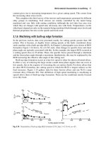
Fig. 1. The example from Cuesta-Albertos et al.: 20 outliers are added to a sample of 600
observations. Top right panel shows the contour plot of the density estimate and the m

0
= 200
(circled) observations belonging to the starting subset. Bottom left panel reports the monitor-
ing plot of (5) for m = 520, ,620. The 95% ellipses of the mixture components fitted to S
600
are plotted in the last panel.
atypical of a mixture of K normal populations, P
1
, ,P
K
, on the basis of a set of m
observations {x
hk
;h = 1, ,m
k
,k = 1, ,K}, where x
hk
are known to come from P
k
and

K
k=1
m
k
= m. The problem is tackled by assessing how typical the observation
is of each P
k
in turn.
In case of unclassified data {x

j
; j = 1, ,m} – like the one considered in the
present paper – McLachlan and Basford suggest that the m observations should be
first clustered by fitting a K-component heteroscedastic normal mixture model. Then,
the aforementioned comparison of the tested observation to each of the mixture com-
ponents in turn is applied to the resulting K clusters as if they represent a “true clas-
sification" of the data. The approach is based on the following distributional results,
which are derived under the assumption that model (1) is valid:
for the generic sample observation x
j
, the quantity
108 Daniela G. Calò
(
Q
k
m
k
d
)D(x
j
;ˆz
k
,
ˆ
6
k
)
(Q
k
+ d)(m

k
−1) −m
k
D(x
j
;ˆz
k
,
ˆ
6
k
)
(6)
has the F
d,Q
k
distribution, where D(x
j
;ˆz
k
,
ˆ
6
k
)=(x
j
− ˆz
k
)
T

ˆ
6
−1
k
(x
j
− ˆz
k
) denotes the
squared Mahalanobis distance of x
j
from the k-th cluster, m
k
is the number of obser-
vations put in the kth cluster by the estimated mixture model and Q
k
= m
k
−d −1,
with k = 1, ,K;
for a new unclassified observation y, the quantity
m
k
(Q
k
+ 1)
(m
k
+ 1)d(Q
k

+ d)
D(y;ˆz
k
,
ˆ
6
k
) (7)
has the F
d,Q
k
+1
distribution, where D(y;ˆz
k
,
ˆ
6
k
) denotes the squared Mahalanobis dis-
tance of y from the k-th cluster, and Q
k
and m
k
are defined as before, with k = 1, ,K.
Therefore, an assessment of how typical an observation z is of the k-th component
of the mixture is given by the tail area to the right of the observed value of (6) or
(7) under the F distribution with the appropriate degrees of freedom, depending on
whether z belongs to the sample (z = x
j
) or not (z = y). Finally, if a

k
(z) denotes this
tail area, z is assessed as being atypical of the mixture if
a(z)= max
k=1, ,K
a
k
(z) ≤ D, (8)
where D is some specified threshold. According to rule (8), z will be labelled as
outlying of the mixture if it is outlying of all the mixture components. The value of
D depends on how the presence of apparently atypical observations is handled: the
more protection is desired against the possible presence of outliers, the higher the
value of D.
We present a FS algorithm using the typicality index a(z) as a measure of “close-
ness" of a generic observation z to the fitted mixture model. For the sake of simplicity,
the same criterion for selecting S
m
0
described in Section 3 is employed. Then, at each
step of the search, a K-component normal mixture model is fitted to the current sub-
set S
m
and the typicality index is computed for each observation x
i
(i = 1, ,n) by
means of (6) or (7), depending on whether the observation is an element of S
m
or an
element of the remainder of the sample in step m. Then, observations are sorted in
decreasing order of typicality: denoting by x

[i],m
the observation with the i-th ordered
typicality value (computed on subset S
m
), subset S
m
is updated as the set of the m+ 1
most typical observations: S
m+1
= {x
[i],m
: i = 1, ,m+ 1}.
If the least typical observation in the newly created subset, that is x
[m+1],m
,is
assessed as being atypical according to rule (8), then the search stops: the tested ob-
servation is nominated as an outlier, together with all the observations not included
in the subset. The performance of the FS-procedure based on the “inferential" ap-
proach has been compared with that of an outlier detection method for clustering
in the presence of outliers (Hardin and Rocke, 2004). The method starts from a ro-
bust clustering of the data and involves a testing procedure about the outlyingness
of the data, which exploits a distributional result for squared Mahalanobis distances
Mixture Models in Forward Search Methods for Outlier Detection 109
based on minimum covariance determinant estimates of location and shape param-
eters. The comparison has been carried out on a simulation experiment reported in
Hardin and Rocke’s paper, with N = 100 independent replicates. In d=4 dimensions,
two groups of 300 observations each are simulated from N(0, I) and N(2c1,I), re-
spectively, where c =

F

2
d;0.99
/d and 1 is a vector of d ones. Sixty outliers stemming
from N(4c1, I) are planted to each dataset, thus placing the cluster of outliers at the
same distance the clean clusters are separated. By separating two clusters of stan-
dard normal data at a distance of 2c, we have clusters that do not overlap with high
probability. The following measures of performance have been used:
A =

N
j=1
Out
j
Nn
out
, B =

N
j=1
TrueOut
j
Nn
out
, (9)
where n
out
=60 is the number of planted outliers and Out
j
(TrueOut
j

) is the number
of observations (planted outliers) declared as outliers in the j-th replicate. Perfect
performance occurs when A = B = 1.
Table 1. Results of the simulation experiment. In both the compared procedures D = 0.01.
The first row is taken from Hardin and Rocke’s paper.
Technique Measures of performance
(A −1) ·100 (B −1) ·100
Hardin and Rocke 4.03 -0.17
FS-based 0.01 -0.05
In Table 1 the measures of performance are given in terms of distance from 1.
Both the methods identify all the planted outliers in nearly all replicates. However,
Hardin and Rocke’s technique seems to have some tendency in identifying a non-
planted observation as an outlier. The FS-based method performs generally better,
probably because it exploits the normality assumption on the components of the
parental mixture density, by means of the typicality measure a(·). It is expected to
be preferable also in case of highly overlapping mixture components, since Hardin
and Rocke’s algorithm may fail for clusters with significant overlap - as the Authors
themselves point out.
5 Concluding remarks and open issues
One critical aspect of the proposed procedure (and of any FS method, indeed) is the
choice of the size m
0
of the initial subset: it should be relatively small so as to avoid
the initial inclusion of outliers, but also large enough to make stable estimates of the
mixture parameters. Moreover, McLachlan and Basford’s test for outlier detection
is known to have poor control over the overall significance level; we dealt with the
110 Daniela G. Calò
problem by using Bonferroni bounds. The test for outlier detection from a mixture
proposed by Wang et al. (1997) does not suffer from this drawback but requires boot-
strap techniques, thus its use in the FS algorithm would increase the computational

burden of the whole procedure.
FS methods are naturally computer-intensive methods. In our FS algorithm, time
savings could come from using the estimation results of step m as an initial value for
the EM in step m +1. A possible drawback of this solution is that the results of one
step irreversibly influence the following ones. The problem of improving computa-
tional efficiency while preserving effectiveness deserves further attention. Finally,
we assume that the number of mixture components, K, is both fixed and known. In
our experience, the first assumption seems to be not crucial: when subset S
0
does not
contain data from one component, say g,thefirst observation from g may be sig-
nalled by the forward plot, but it can’t appear like an outlier since its inclusion does
not occur in the final steps of the search. On the contrary, generalizing the procedure
for K unknown is a rather challenging task, which we are presently working on.
References
ATKINSON, A.C. (1993): Stalactite plots and robust estimation for the detection of multivari-
ate outliers. In: E. Ronchetti, E. Morgenthaler, and W. Stahel (Eds.): New Directions in
Statistical Data Analysis and Robustenss., Birkhäuser, Basel.
ATKINSON, A.C., RIANI, C. and CERIOLI A. (2004): Exploring Multivariate Data with the
Forward Search. Springer, New York.
FRALEY, C. and RAFTERY, A.E. (1998): How may clusters? Which clustering method?
Answers via model-based cluster analysis. The Computer Journal, 41, 578-588.
HADI, A.S. (1994): A modification of a method for the detection of outliers in multivariate
samples. J R Stat Soc, Ser B, 56, 393-396.
HARDIN, J. and ROCKE D.M. (2004): Outlier detection in the multiple cluster setting us-
ing the minimum covariance determinant estimator. Computational Statistics and Data
Analysis, 44, 625-638.
HENNIG, C. (2004): Breakdown point for maximum likelihood estimators of location-scale
mixtures. The Annals of Statistics, 32, 1313-1340.
MCLACHLAN, G.J. and BASFORD K.E. (1988): Mixture Models: Inference and Applica-

tions to Clustering. Marcel Dekker, New York.
MCLACHLAN, G.J. and PEEL, D. (2000): Finite Mixture Models. Wiley, New York.
WANG S. et al. (1997): A new test for outlier detection from a multivariate mixture distribu-
tion, Journal of Computational and Graphical Statistics, 6, 285-299.
On Multiple Imputation Through Finite Gaussian
Mixture Models
Marco Di Zio and Ugo Guarnera
Istituto Nazionale di Statistica,
via Cesare Balbo 16, 00184 Roma, Italy
{dizio, guarnera}@istat.it
Abstract. Multiple Imputation is a frequently used method for dealing with partial nonre-
sponse. In this paper the use of finite Gaussian mixture models for multiple imputation in a
Bayesian setting is discussed. Simulation studies are illustrated in order to show performances
of the proposed method.
1 Introduction
Imputation is a common approach to deal with nonresponse in surveys. It consists
in substituting missing items with plausible values. This approach has been widely
used because it allows to work with a complete data set so that standard analysis can
be applied. Despite of this important advantage, the introduction of imputed values
is not a neutral task. In fact, imputed values are not really observed and this should
be explicitly taken into account in statistical inference based on the completed data
set. If standard methods are applied as if the imputed values were really observed,
there would be a general overestimate of the precision of the results, resulting, for
instance, in too narrow confidence intervals. Multiple imputation (Rubin, (1987)) is
a methodology for dealing with this problem. It essentially consists in imputing a
certain number of times the incomplete data set following specific rules. The result-
ing completed data set is analysed by standard methods and results are combined in
order to yield estimates and assessing their precision including the additional source
of variability due to nonresponse. The multiplicity of completed data sets has the
role of reflecting the variability due to the imputation mechanism. Although in mul-

tiple imputation data normality is frequently assumed, this assumption does not fit
all situations (e.g., multimodal distributions). Moreover, the analyst who works on
the completed data set not necessarily will or must be aware of the model used for
imputation. Thus, problems may arise when the models used by the analyst and by
the imputer are different. Meng (1994) suggests to use a model for imputation that
is reasonably accurate and general to overcome this difficulty. To this aim, an in-
teresting work is that of Paddock (2002) who proposes a nonparametric multiple
imputation technique based on Polya trees. This technique is appealing since it al-
112 Marco Di Zio and Ugo Guarnera
lows to treat continuous and ordinal data, and in some circumstances also categorical
variables. However, in Paddok’s paper it is shown that, even with nonnormal data, in
some case the technique based on normality is still quite better. Nonnormal data can
be dealt with by using finite mixtures of Gaussian distributions (GMM) since they
are flexible enough to approximate a wide class of density functions with a limited
number of parameters. These models can be seen as generalizations of the general
location model used by Little and Rubin (2002) to model partially observed data
with mixed categorical and continuous variables. Unlike in the latter case, however,
in the present approach categorical variables are latent variables (‘class labels’ that
are never observed), and their role is merely to allow better approximation of the
true data distribution. The performance of GMM in a likelihood based approach for
single imputation is evaluated in Di Zio et al. (2007). In this paper we discuss the
use of finite mixtures of Gaussian distributions for multiple imputation in a Bayesian
framework. The paper is structured as follows. Section 2 describes multiple impu-
tation through mixture models. In Section 3, the problem of label switching is dis-
cussed. Section 4 is devoted to the description and discussion of the experiments
carried out in order to assess the performance of the proposed method.
2 Multiple imputation
Multiple imputation has been proposed for both frequentist and Bayesian analy-
ses. Nevertheless, the theoretical justification is most easily understood from the
Bayesian perspective. In this setting, the ultimate goal is to fill in missing values

Y
mis
with values y
mis
drawn from the predictive distribution that, once an appropri-
ate prior distribution for ) is set, can be written as
P(Y
mis
|y
obs
)=

P(Y
mis
|y
obs
,))P()|y
obs
)d) (1)
where Y
mis
are the missing values and Y
obs
the observed ones. The imputation
process is repeated m times, so m completed data sets are obtained. These m dif-
ferent data sets incorporate the uncertainty about the missing imputed values. Let
us suppose that Q(Y) is the quantity of interest, e.g., a population mean, and that
an estimate
ˆ
Q(Y)

(i)
is computed on the ith completed data set, for i = 1, ,m.
The final estimate
ˆ
Q is defined by
ˆ
Q =
1
m

m
i=1
ˆ
Q(Y)
(i)
. The estimate
ˆ
T of the
variance of
ˆ
Q can be obtained by combining a within component term
ˆ
U and a
between component term
ˆ
B. The former is the average of the m standard vari-
ance estimates
ˆ
U
(i)

for complete data computed on the ith completed data set, for
i = 1, ,m:
ˆ
U =
1
m

m
i=1
ˆ
U
(i)
. The between variance is the variance of the m esti-
mates, i.e.
ˆ
B =
1
m−1

m
i=1
(
ˆ
Q
(i)
−
ˆ
Q)
2
. Finally, the total variance of

ˆ
Q is estimated by
ˆ
T =
ˆ
U +(1+m
−1
)
ˆ
B, and a 95% confidence interval for Q is given by
ˆ
Q±t
Q,0.975
ˆ
T
1/2
,
where the degrees of freedom are Q =(m−1){1 +[(1 + m
−1
)
ˆ
B]
−1
ˆ
U}, (see Rubin,
1987).
On Multiple Imputation Through Finite Gaussian Mixture Models 113
Since it is often difficult to obtain a closed form for the observed posterior distri-
bution P()|y
obs

), the data augmentation algorithm may be used (Tanner and Wong,
1987). This algorithm consists of iterating the two following steps:
1. I-step - draw
˜
y
mis
from P(Y
mis
|y
obs
,
˜
))
2. P-step - draw
˜
) from P()|
˜
y
mis
,y
obs
).
This is a Gibbs sampling algorithm and, after convergence, the resulting sequence of
values
˜
y
mis
can be thought of as generated from P(Y
mis
|y

obs
). Data augmentation is
explicitly described by Schafer (1997) when data follow a Gaussian distribution. We
study the case when data are generated from a finite mixture of K Gaussian distribu-
tions, i.e., when each observation y
i
for i = 1, ,n is supposed to be a realization of
a p-dimensional r.v. Y
i
with density:
f (y
i
|))=
K

k=1
S
k
N
p
(y
i
|T
k
), y ∈R
p
where

k
S

k
= 1,S
k
≥ 0fork = 1, ,K,andN
p
(y
i
|T
k
) is the Gaussian density
with parameters T
k
=(z
k
,6
k
). Note that ) denotes the full set of parameters: ) =
(S
1
, S
K
;T
1
, ,T
K
).
Mixture models have a natural missing data formulation if we suppose that each
observation y
i
comes from a specific but unknown component k of the mixture, and

introduce, for each unit i, an indicator or allocation variable Z
i
, taking values in
{
1, ,K
}
, with z
i
= k if individual i belongs to group k. The discrete variables Z
i
are
independently distributed according to P(Z
i
= k|))=S
k
, (i = 1, ,n;k = 1, ,K).
Furthermore, conditional on Z
i
= k, the observations y
i
are supposed to be i.i.d. from
the density N
p
(y
i
|T
k
). Thus, if some items are missing for the ith unit, the relevant
distribution, conditional on Z
i

= k,isP(Y
mis
|y
obs
,T
k
), while the classification prob-
abilities, expressed in terms of y
i,obs
,are:
W
gi
= P(Z
i
= g|y
i,obs
,))=
S
g
N
p
(y
i,obs
|T
g
)

K
k=1
S

k
N
p
(y
i,obs
|T
k
)
, g = 1, ,K (2)
where N
p
(y
i,obs
|T
g
) is the Gaussian marginal distribution of the gth mixture compo-
nent of the variables observed in the ith unit.
The previous formulation leads to a data augmentation algorithm consisting, at
the tth iteration, of the following two steps:
• I-step: for i = 1, ,n
– draw a random value of the allocation variable z
(t)
i
from the distribution
P(Z
i
|y
i,obs
,)
(t−1)

), i.e., select a value in
{
1, ,K
}
using the probabilities
W
1i
, ,W
Ki
defined in formula (2) expressed in terms of the current value of
vector )
(t−1)
;
–drawy
(t)
i,mis
(the missing part of the ith vector y
(t)
i
) from P(y
i,mis
|z
(t)
i
,y
i,obs
,)
(t)
).
•P-step:

draw )
(t)
from the distribution P()|y
obs
,y
(t)
mis
).
114 Marco Di Zio and Ugo Guarnera
The above scheme produces a sequence (z
(t)
,y
(t)
mis
,)
(t)
) which is a Markov chain
with stationary distribution P(Z,Y
mis
,)|y
obs
). The convergence properties of the al-
gorithm have been studied by Diebolt and Robert (1994) in the case of completely
observed data.
The choice of an appropriate prior is a critical issue in Gaussian mixture models.
For instance, reference priors lead to improper priors for the specific component
parameters that are independent across the mixture components. This situation is
problematic insofar posterior distributions remain improper for configurations where
no units are assigned to some components. In this paper we follow a hierarchical
Bayesian approach, based on weakly informative priors, as introduced by Richardson

and Green (1997) for univariate mixtures, and generalized to the multivariate case
by Stephen (2000). In this approach it is assumed that the prior distribution for z
k
is
rather flat over an interval of variation of the data. The hierarchical structure of the
prior distributions for a K-component p-variate Gaussian mixture is given by:
z
k
∼ N([,<
−1
)
6
−1
k
|E ∼ W(2D, (2E)
−1
)
E ∼ W(2G, (2h)
−1
)
S ∼ D(J),
where W and D denote the Wishart and Dirichlet distributions respectively, and the
hyperparameters [, <, D, G, h, J, are constants defined below. Let R
j
be the length
of the observed interval of variation (range) of the obtained valu s for the vari-
able Y
j
,and[
j

the corresponding midpoint ( j = 1, ,p). Then, [ is the p-vector:
([
1
, ,[
p
), while the matrix < is the diagonal matrix whose element \
jj
is R
−2
j
.
The other hyperparameters are specified as follows:
D = p +1, G = D/10, h = 10<, J =(1, ,1).
The P-step described in general above in this section, with )
(t)
=
(E
(t)
,S
(t)
1
, ,S
(t)
K
;z
(t)
1
, ,z
(t)
K

;6
(t)
1
, ,6
(t)
K
) can be implemented by sampling from
the appropriate posterior distributions as follows:
E
(t+1)
|···∼W

2G +2gD,(2h+ 2
K

k=1
6
(t)
−1
k
)
−1

,
S
(t+1)
|···∼D(J+ n
1
, ,J +n
K

),
z
(t+1)
k
|···∼N

(n
k
6
(t)
−1
k
+ <)
−1
(n
k
6
(t)
−1
k
y
k
+ <[),(n
k
6
(t)
−1
k
+ <)
−1


,
6
−1(t+1)
k
|···∼W
⎛
⎝
2D +n
k
,(2E
(t+1)
+

i:z
i
=k
(y
i
−z
(t+1)
k
)(y
i
−z
(t+1)
k
)

)

−1
⎞
⎠
,
where |··· denotes conditioning on all other variables. In the previous formulas n
k
denotes the number of units assigned to the k
th
mixture component at the t
th
step,
and
y
k
is the mean:

i:z
i
=k
y
i
/n
k
.
On Multiple Imputation Through Finite Gaussian Mixture Models 115
3 Label switching
Label switching is a typical problem in Bayesian estimation of finite mixture mod-
els (Stephens, (2000)). When using symmetric priors (i.e., invariant with respect
to permutations of the components), the posterior distributions are still symmet-
ric and thus the marginal posterior distributions for the parameters will be identi-

cal for all the mixture components. Inference based on MCMC is meaningless, be-
cause it results in averaging over different mixture components. Nevertheless, this
problem does not affect inference on parameters that are independent of label com-
ponents. For instance, if the parameter to be estimated is the population mean, as
often required in official statistics, the target quantity is independent of the com-
ponent labels. Moreover, in multiple imputation, the estimate is computed on the
observed and imputed values, and the imputed values are drawn from P(Y
mis
|y
obs
)
that is invariant with respect to permutation of component labels. As an illustra-
tive example, we have drawn 200 random samples from the two-component mixture
f (y)=0.5N(1.3,0.1)+0.5N(2,0.15) in R
1
, and nonresponse is artificially intro-
duced with a 20% missing rate. This dataset is multiply imputed according to the
algorithm previously described. In Figure 1 the trace plot of the component means
obtained via data augmentation, and of the sample mean that is used to produce mul-
tiple imputation estimates are shown (5000 iterations). In the figure, the component
means of the generating mixture distribution (dashed lines) are also reported. More-
over vertical lines, corresponding to label switching, are depicted. It is worth to note
that the label switching of the component means does not affect the target estimate
that in fact is stable.
0 1000 2000 3000 4000 5000
0.0 1.0 2.0 3.0
DA iteration
mu1
0 1000 2000 3000 4000 5000
0.0 1.0 2.0 3.0

DA iteration
mu2
0 1000 2000 3000 4000 5000
0.0 1.0 2.0 3.0
DA iteration
sample mean
Fig. 1. Trace plot of the two-component means and the sample means computed through the
data augmentation algorithm.
116 Marco Di Zio and Ugo Guarnera
4 Simulation study and results
We present a simulation study to assess the performance of Bayesian GMM for mul-
tiple imputation. In order to mimic the situtation in official statistics, a sample of
N = 50000 units (representing the finite population) with three variables (Y
1
,Y
2
,Y
3
)
is drawn from a probability model. The target parameter is the mean of the variables
in the finite population. A random sample u without replacement of n = 1000 units is
drawn from the reference population. This sample is corrupted by the introduction of
missing values according to a Missing at Random mechanism (MAR). Missing items
are introduced for the variables (Y
2
,Y
3
) depending on the observed values y
1
of the

variable Y
1
under the assumption that the higher the value of Y
1
the higher is the
nonresponse propensity. Denoting by q
i
the ith quartile of the empirical distribution
of Y
1
, the nonresponse probabilities for (Y
2
,Y
3
) are 0.1 if y
1
< q
1
, 0.2 if y
1
∈[q
1
,q
2
),
0.4 if y
1
∈ [q
2
,q

3
) and 0.5 if y
1
≥ q
3
.
The sample u is multiply imputed (m=5) via GMM. Data augmentation algorithm
is initialized by using maximum likelihood estimates (MLE) obtained through the
EM algorithm as described in Di Zio et al. (2007). After a burn-in period of 500 iter-
ations, multiple imputation is performed by subsampling the chain every t iterations,
that is, the Y
mis
used for imputation are those referring to the iterations (t, 2t, ,5t).
Subsampling is used to avoid dependent samples, as suggested by Schafer (1997).
Although the burn-in period may appear to be not very long, as again suggested by
Schafer (1997), the initialization of the algorithm with a good starting point (e.g.,
through MLE) may speed up the convergence of the chain. This is also confirmed by
analysing the trace plot of the parameters.
Once the data set is imputed, for each analysed variable, the estimate of the mean,
its variance, and the corresponding 95% confidence interval for the mean are com-
puted by applying the multiple imputation formulas to the usual Horvitz-Thompson
estimator
ˆ
¯
Y = ¯y, and to its estimated variance

Var(
ˆ
¯
Y)=(

1
n
−
1
N
)s
2
, where s
2
is the
sample variance. The estimates are compared to the true mean value of the popu-
lation by computing the square difference, and verifying whether the true value is
included in the confidence interval. Taking the population fixed, the experiment is
repeated 1000 times, and the results are averaged over these iterations. The results
give simulated MSE, bias, simulated coverage corresponding to a 95% nominal level,
and average length of the confidence intervals.
This simulation scheme is applied in two settings. In the first, the population is
drawn from a two-component Gaussian mixture, with mixing parameter S = 0.75,
mean vectors z
1
=(0,0, 0)

, z
2
=(3,5,8)

, and covariance matrices
6
1
=

⎛
⎝
3.02.42.4
2.43.02.1
2.42.11.3
⎞
⎠
, 6
2
=
⎛
⎝
4.02.42.4
2.43.52.1
2.42.13.2
⎞
⎠
.
In the second setting, the population is generated from the Cheriyan and Ram-
abhadran’s multivariate Gamma distribution described in Kotz et al. (2000) pp. 454-
456. In order to draw a sample of a 3-variate random vector (Y
1
,Y
2
,Y
3
) from such
On Multiple Imputation Through Finite Gaussian Mixture Models 117
a distribution the following procedure is adopted. First, we consider 4 independent
random variables X

i
in R
1
for i = 0,1,2,3 that are distributed according to Gamma
distributions characterised by different parameters T
i
. Then, the 3-variate random
vector is obtained combining the X
i
so that Y
i
= X
0
+ X
i
for i = 1,2,3. The values of
the parameters are T =(1,0.2,0.2,0.4)

.
In the two-component Gaussian mixture population, multiple imputation is car-
ried out according to a plain normal model (hereafter NM) and a mixture of two
Gaussian components (M
2
). The results for the variable Y
3
are illustrated in Table
1. For the Gamma population, multiple imputation is performed by using the plain
normal model (NM)andaK-component mixture M
K
for K = 2, 3, 4. Results for the

variable Y
3
are provided in Table 2.
Table 1. Results of the experiment where population is based on a two-component Gaussian
mixture
Mod bias MSE S.Cov Length
NM -0.0144 0.1323 93.7% 0.5000
M
2
0.0014 0.1316 94.9% 0.5163
Table 2. Results of the experiment where population is based on Multivariate Gamma
Mod bias MSE S.Cov Length
NM 0.0015 0.0431 93.8% 0.1604
M
2
0.0052 0.0437 94.0% 0.1661
M
3
0.0043 0.0435 94.0% 0.1651
M
4
0.0059 0.0442 94.1% 0.1655
Results show that confidence intervals are close to the nominal coverage. In par-
ticular, in the first experiment, the confidence interval computed by the mixture mod-
els is better than that computed through a Gaussian distribution. The improvement
is due to the fact that the model used for estimation is correctly specified. This sug-
gests the need of improving estimation of unknown distribution by means of mixture
models. To this aim it could be an important step to consider the number of mixture
components as a random variable, thus incorporating the model uncertainty in the
estimation phase.

References
DIEBOLT, J. and ROBERT, C.P. (1994): Estimation of finite mixture distributions through
Bayesian sampling. Journal of the Royal Statistical Society B, 56, 363–375.
118 Marco Di Zio and Ugo Guarnera
DI ZIO, M., GUARNERA, U. and LUZI, O. (2007): Imputation through finite Gaussian mix-
ture models. Computational Statistics and Data Analysis, 51, 5305–5316.
KOTZ, S., BALAKRISHNAN, N. and JOHNSON, N.L. (2000): Continuous multivariate dis-
tributions. Vol.1, 2nd ed. Wiley, New York.
LITTLE, R.J.A. and RUBIN, D.B. (2002): Statistical analysis with missing data. Wiley, New
York.
MENG, X.L. (1994): Multiple-imputation inferences with uncongenial sources of input (with
discussion). Statistical Science, 9, 538–558.
PADDOCK, S.M. (2002): Bayesian nonparametric multiple imputation of partially observed
data with ignorable nonresponse. Biometrika, 89, 529–538.
RICHARDSON, S. and GREEN, P.J. (1997): On Bayesian analysis of mixtures with an un-
known number of components.Journal of the Royal Statistical Society B, 59, 731–792.
RUBIN, D.B. (1987): Multiple imputation for nonresponse in surveys. Wiley, New York.
SCHAFER, J.L. (1997): Analysis of incomplete multivariate data. Chapman & Hall, London.
STEPHENS, M. (2000): Bayesian analysis of mixture models with an unknown number of
components-an alternative to reversible jump methods. Annals of Statistics, 28, 40–74.
TANNER, M.A. and WONG, W.H. (1987): The calculation of posterior distribution by data
augmentation (with discussion). Journal of the American Statistical Association, 82,
528–550.
Rationale Models for Conceptual Modeling
Sina Lehrmann and Werner Esswein
Dresden University of Technology, Chair of Information Systems, esp. Systems Engineering,
01062 Dresden, Germany
{sina.lehrmann, werner.esswein}@tu-dresden.de
Abstract. In developing information systems conceptual models are used for varied purposes.
Since the modeling process is characterized by interpretation and abstracting the situation at

hand it is essential to enclose information about the design process the modelers went through.
This aspect is often discarded. But the lack of this information hinders the reuse of past knowl-
edge for later, similar problems encountered and supports the repeat of failures.
The design rationale approaches, discussed in the software engineering community since
the 1990s, seem to be an effective means to solve these problems. But the semiformal style of
the rationale models challenges the retrieval of the relevant information. The paper explores
an approach for classifying issues by its responding alternatives as an access to the complex
rationale documentation.
1 Subjectivism in the modeling process
Our considerations are based on a moderate constructivistic position. This attitude of
mind has significant consequences on the design of the modeling process as well as
on the evaluation of the quality of the resulting model. As it is outlined in (Schütte
and Rotthowe (1998)) a model is a result of a cognitive process done by a modeler,
who is structuring the considered system according to a specific purpose. Because
of the differing thought patterns of the stakeholder a consensus about structuring the
problem domain as well as about the model representation has to be defined. In this
way the modeling process is a consensus oriented one.
The definition of the application domain terms is an accepted starting point for
the process of conceptual modeling (cp. Holten (2003), p. 201). Therefore it is fair
to assume that no misinterpretation of the applied terminology occurs.
In order to manage the subjectivity in the modeling process and to support the
traceability of the conceptualizations done by the model designer, S
CHUETTE and
R
OTTHOWE proposed the Guidelines of Modeling as generic modeling conventions
(cp. Schütte and Rotthowe (1998)). In doing so they also considered not only the
significant role of the model designer but also the role of the model user. They claim
that the model user is only able to interpret the model in a correct way, if he knows
156 Sina Lehrmann and Werner Esswein
the underlying guidelines of the model design (cp. Schütte and Rotthowe (1998), p.

242).
Model designers are facing similar problems in different projects (cp. Fowler
(1997)). Owing to a lack of an explicit and maintained knowledge base containing
experiences in model construction and model use, similar problems are solved re-
peatedly at higher costs than they have to be (cp. Hordijk and Wieringa (2006), p.
353).
Due to the subjectivism in the modeling process it is inevitable to externalize the
assumptions and objectives the model bases on. The traceability of the model con-
struction is not only relevant for reusing modeling solutions but also for maintaining
the model itself. Stakeholder, who were not involved in the modeling process, are
not able to interpret the model in the right way. Particularly with regard to fractional
changes of the model, the lack of rationale information could have far-reaching con-
sequences like violating assumptions, constraints or tradeoffs.
Argumentation based models of design rationale ought to be suitable for solv-
ing these problems (cp. Dutoit et al. (2006)). Based on the literature about Design
Rationale approaches in Software Engineering we derive an approach for reusing
experiences in conceptual modeling. For this purpose we use the classification of
rationale fragments accessing different rationale models resulting from various mod-
eling projects.
2 The design rationale approach
According to the latest level of knowledge in software engineering issue models
which represent the justification for a design in a semiformal manner are the most
promising approach to solve the problems described above (cp. Dutoit et al. (2006)).
They could be used for structuring the rationale in a more systematic way than text
documentations do. In addition, implementing a knowledge base containing the ra-
tionales of past modeling projects could improve the efficiency of future modeling
processes as well as the quality of the outcoming artifacts.
VAN D ER VEN ET AL. identified a general process for creating rationale, which
most of the approaches have in common (cp. van der Ven et al. (2006), p. 333).
After the problems are identified and described in problem statements they are

evaluated one by one. Alternative solutions are created, evaluated and weighted for
their suitability of solving the problem at hand. After an informed decision is made,
it is documented along with its justification in a rationale document.
Various approaches for capturing design rationale have been evolved. Most of
them are basing on very similar concepts and are more or less restrictive. For our
concerns we have chosen the QOC notation, because it is quite expressive and deals
directly with evaluation of artifact features (cp. Dutoit et al. (2006), p. 13).
2.1 The QOC-Notation
The Questions, Options, and Criteria (QOC) notation is used for the design space
analysis, which
¨
’ [ ] creates an explicit representation of a structured space of design
Rationale Models for Conceptual Modeling 157
alternatives and the considerations for choosing among them [ ]
¨
’ (MacLean et al.
(1991), p. 203).
QOC is a semiformal node-and-link diagram. Though it provides a formal struc-
ture, the statements within any of the nodes are informal and unrestricted. M
ACLEAN
ET AL
.define the three basic concepts, questions, options, and criteria. These con-
cepts and their relations are depicted in Figure 1.
Fig. 1. QOC notation
Questions represent key issues of design decisions not having trivial solutions.
They are means for structuring the design space of an artifact. Options are alternative
solutions responding to a question.
¨
’ [ ] Criteria represent the desirable properties
of the artifact and requirements that it must satisfy [ ]

¨
’ (MacLean et al. (1991), p.
208). Because they state the objectives of the design in a clear and structured manner,
they form the basis of evaluation, weighting and selection of a design solution. The
labeled link between an option and a criterion displays the assessment whether an
option satisfy a criterion. In doing so tradeoffs are made explicit and the discussion
about choosing among the options turns focus to the purpose the design is made for.
The presented design space analysis is an argumentation based approach. On this
account all of the QOC elements could be supported or challenged by arguments.
These arguments could play an important role for the evolution of the organizational
knowledge base. In the case of reusing design solution the validity of the arguments
the primary design decision was based on has to be proven.
One objection to the utility of rationale models is that they are very complex
and hardly to manage without any tool support (cp. MacLean et al. (1991), p. 216).
Due to the complexity of the rationale models it is necessary to provide an effective
retrieval mechanism. Otherwise this kind of documentation seems to be useless for a
managed organizational memory.
158 Sina Lehrmann and Werner Esswein
2.2 Reuse of rationale documentation
Since the capturing of design rationale takes considerable effort, the benefit from
using the resulting models has to exceed the costs of their construction.
H
ORDIJK and WIERINGA propose Reusable Rationale Blocks for reusing design
knowledge in order to improve quality and efficiency of design choices (cp. Hordijk
and Wieringa (2006)). For achieving this goal they use generalized pieces of decision
rationale.
The idea of Reusable Rationale Blocks bases on the QOC approach and on
the concept of design patterns. Design Patterns are widely accepted approaches for
reusing design knowledge. Though they provide a detailed description of a solu-
tion for a repeating design problem, they lack evaluations of alternative solutions

(cp. Hordijk and Wieringa (2006), p. 356). But they are appropriate options within
a QOC-Model, which could be ranked by a set of quality indicators. In this way
tradeoffs and dependencies among solutions can be considered.
In order to define appropriate patterns and to assemble an experience base the
documented argumentation, i.e. the rationale models, has to be analyzed. To support
the analysis of the rationale documentation of several modeling projects an effective
and efficient access is needed. This goal claims that all relevant information to the
problem at hand is retrieved and no irrelevant information is element of the answer
set. Precision and recall are accepted measures for assessing the achievement of this
objective.
The classification scheme presented in the next section could be regarded as an
intermediate stage for editing the rationale information of project specific documen-
tations to generate generic rationale information like the described Reusable Ratio-
nale Blocks.
3 Classification of rationale fragments
The QOC notation is more restrictive than most of the other approaches and deals
directly with the evaluation of artifact features. These are premises for classifying
the options of divers rationale models as a systematic entry to the rationale docu-
mentation.
To depict our idea we use F
OWLERS Analysis Pattern (cp. Fowler (1997)). He
discusses different alternatives for modeling derivatives.
Rationale Models for Conceptual Modeling 159
Short
Contract
Long
(a) Subtyping
Contract
isLong
(b) Boolean Attribute

Fig. 2. Alternative Modeling of Long and Short
Figure 2 shows two different models of a contract and the distinction between
Long and Short. In the first model subtyping is used for this purpose whereas the
second one uses the Boolean attribute isLong.F
OWLER states that both alternatives
are equivalent in conceptual modeling (cp. Fowler (1997), p. 177).
Fig. 3. Different Structures of the Optionality of a Contract
For modeling the concept Option FOWLER presents two alternatives depicted in
Figure 3 (cp. Fowler (1997), pp. 200ff.). In the first model the optionality of a contract
is represented by subtyping. In this way an option is a t’"[ ] kind of contract with
additional properties and some variant behavior [ ]t’" (Fowler (1997), p. 204). The
second model differentiates between an option and its underlying base contract. Even
F
OWLER can give only little advice for choosing among these alternative modeling
solutions.
160 Sina Lehrmann and Werner Esswein
Fig. 4. Example for a Design Space Analysis
For this purpose we analyzed the rationale for the modeling alternatives pre-
sented by F
OWLER. Figure 4 shows an extract of the rationale model using QOC.
The represented discussion bases on the assumption that there has been a decision
to include the information objects Option, Long and Short in the model. From these
decisions, there follow two Questions concerning the divers alternatives.
On closer examination two different kinds of modeling issues can be derived
from the provided solutions. The first one are problem solutions concerning the use
of modeling grammar and its influence on the resulting model quality. For solving
these problems the knowledge, experiences and assumptions of the modeling expert
are decisive.
As a second kind of issues we can identify questions concerning the structuring
of the considered system. The expertise and the instinct of the domain expert should

dominate this discussion.
A rationale fragment contains at least a question and its associated options, cri-
teria, and arguments. One single question deals either with structuring the problem
domain or with applying the modeling grammar. While the considered options in
the QOC model can be identified by means of the formal structure, the statements
within the nodes are facing the common problems of information retrieval. If we can
presume a defined terminology both of the application domain and of the modeling
grammar a classification of the Options can identify Questions concerning similar
design problems discussed in several rationale models. The resulting classification
can be used as a starting point for the analysis of the archived rationale documenta-
tion in order to accumulate and aggregate the specific project experiences.
To exemplify our thoughts Figure 5 depicts a possible classification of rationale
fragments. The two main branches, problem domain and modeling grammar, catego-
rize the rationale information according to the experiences of the domain expert and
the modeling expert respectively.
The differentiation between these two kinds of modeling issues is also reflected
in the two principles of the Guidelines of Modeling, construction adequacy and lan-
guage suitability (cp. Schütte and Rotthowe (1998), p. 246). Just these principles