Data Analysis Machine Learning and Applications Episode 1 Part 8 ppsx

Rationale Models for Conceptual Modeling 161
Fig. 5. Classification of Rationale Fragments
reveal that information modeling is characterized by various decision problems. So
the choice of the information objects, relevant for the modeling problem, determines
the appropriateness of the resulting model. Furthermore an agreement about the ap-
plication of certain modeling techniques has to be settled.
The branch referring to the usability and utility of the modeling grammar de-
serves closer attention. Rationale documentations concerning these kinds of issues
are not only useful for the model designer and user, but they are also invaluable as
feedback information for an incremental knowledge base for the designers of the
modeling method.
Experiences in the method use, i.e. usage of the modeling grammar, are discov-
ered as an essential resource for the method engineering process (cp. Rossi et al.
(2004)). R
OSSI ET AL. stress these kind of information as a complementary part of
the method rationale documentation. They define the method construction rationale
and the method use rationale as a coherent unit of rationale information.
4 Conclusion
The paper suggests that a classification of design rationale fragments can support the
analysis and reuse of modeling experiences resulting in an explicit and systematic
structured organizational memory.
Owing to the subjectivism in the modeling process the application of an argumen-
tation based design rationale approach could assist the reasoning in design decisions
and the reflection of the resulting model. Furthermore Reusable Rationale Blocks are
valuable assets for estimating the quality of the prospective conceptual model.
The semiformality of the complex rationale models challenges the retrieval of
documented discussions relevant to a specific modeling problem. The paper presents
an approach for classifying issues by its responding alternatives as a systematic entry
in the rationale models as a starting point for the analysis of modeling experiences.
What is needed now is empirical research on the impact of design rationale mod-
eling on the resulting conceptual model. An appropriate notation has to be elabo-

rated. This is not a trivial mission because of the tradeoff between a flexible model-
162 Sina Lehrmann and Werner Esswein
ing grammar and an effective retrieval mechanism. The more formal a notation is the
more precise the retrieval system works. The other side of the coin is that the more
formal a notation is the more the capturing of rationale information is interfering.
But a high intrusive approach will hardly be used for supporting decision making on
the fly.
References
DUTOIT, A.H., McCALL, R., MISTRIK, I. and PAECH, B. (2006): Rationale Management in
Software Engineering: Concepts and Techniques. In: A.H. Dutoit, R. McCall, I. Mistrík
and B. Paech (Eds.): Rationale Management in Software Engineering. Springer, Berlin,
1–48.
FOWLER, M. (1997): Analysis Patterns: Reusable Object Models, Addison-Wesley, Menlo
Park.
HOLTEN, R. (2003): Integration von Informationssystemen. Theorie und Anwendung im Sup-
ply Chain Management. Habilitationsschrift, Westfälische Wilhelms-Universität Mün-
ster.
HORDIJK, W. and WIERINGA, R. (2006): Reusable Rationale Blocks: Improving Quality
and Efficiency of Design Choices. In: A.H. Dutoit, R. McCall, I. Mistrík and B. Paech
(Eds.): Rationale Management in Software Engineering. Springer, Berlin, 353–370.
MACLEAN, A., YOUNG, R.M., BELLOTTI, V.M.E. and MORAN, T.P. (1991):Questions,
Options and Criteria: Elements of Design Space Analysis. Human-Computer Interaction,
6(1991) 3/4, 201–250.
ROSSI, M., RAMESH, B., LYYTINEN, K. and TOLVANEN, J P. (2004): Managing Evolu-
tionary Method Engineering by Method Rationale. Journal of the Association for Infor-
mation Systems, 5(2004) 9, 356–391.
SCHÜTTE, R. (1999): Architectures for Evaluating the Quality of Information Models - a
Meta and an Object Level Comparison. In: J. Akoka, M. Bouzeghoub, I. Comyn-Wattiau
and E. Métais (Eds.): Conceptual Modeling - ER ’99, 18th International Conference
on Conceptual Modeling, Paris, France, November, 15-18, 1999, Proceedings. Springer,

Berlin, 490–505.
SCHÜTTE, R. and ROTTHOWE, T. (1998): The Guidelines of Modeling - An Approach to
Enhance the Quality in Information Models. In: T.W. Ling, S. Ram and M.L. Lee (Eds.):
Conceptual Modeling - ERt’98, 17th International Conference on Conceptual Modeling,
Singapore, November 16-19, 1998, Proceedings. Springer, Berlin, 240–254.
VAN DER VEN, J.S., JANSEN, A.G.J., NIJHUIS, J.A.G. and BOSCH, J. (2006): Design
Decisions: The Bridge between Rationale and Architecture. In: A.H. Dutoit, R. McCall,
I. Mistrík and B. Paech (Eds.): Rationale Management in Software Engineering. Springer,
Berlin, 329–348.
The Noise Component
in Model-based Cluster Analysis
Christian Hennig
1
and Pietro Coretto
2
1
Department of Statistical Science, University College London,
Gower St, London WC1E 6BT, United Kingdom

2
Dipartimento di Scienze Economiche e Statistiche Universita degli Studi di Salerno
84084 Fisciano - SA - Italy

Abstract. The so-called noise-component has been introduced by Banfield and Raftery
(1993) to improve the robustness of cluster analysis based on the normal mixture model.
The idea is to add a uniform distribution over the convex hull of the data as an additional
mixture component. While this yields good results in many practical applications, there are
some problems with the original proposal: 1) As shown by Hennig (2004), the method is not
breakdown-robust. 2) The original approach doesn’t define a proper ML estimator, and doesn’t
have satisfactory asymptotic properties.

We discuss two alternatives. The first one consists of replacing the uniform distribution
by a fixed constant, modelling an improper uniform distribution that doesn’t depend on the
data. This can be proven to be more robust, though the choice of the involved tuning constant
is tricky. The second alternative is to approximate the ML-estimator of a mixture of normals
with a uniform distribution more precisely than it is done by the “convex hull” approach. The
approaches are compared by simulations and for a real data example.
1 Introduction
Maximum Likelihood (ML)-estimation of a mixture of normal distributions is a
widely used technique for cluster analysis (see, e.g., Fraley and Raftery (1998)).
Banfield and Raftery (1993) introduced the term “model-based cluster analysis” for
such methods.
In the present paper we are concerned with an idea for improving the robustness
of these estimators against outliers and points not belonging to any cluster. For the
sake of simplicity, we only deal with one-dimensional data here, but the theoretical
results carry over easily to multivariate models. See Section 6 for a discussion of
computational issues in the multivariate case.
Observations x
1
, ,x
n
are modelled as i.i.d. according to the density
128 Christian Hennig and Pietro Coretto
f
K
(x)=
s

j=1
S
j

M
a
j
,V
2
j
(x), (1)
where K =(s,a
1
, ,a
s
,V
1
, ,V
s
,S
1
, ,S
s
) is the parameter vector, the number
of components s ∈ IN may be known or unknown, (a
j
,V
j
) pairwise distinct, a
j
∈
IR , V
j
> 0, S

j
> 0, j = 1, ,s,

s
j=1
S
j
= 1andM
a,V
2
is the density of the normal
distribution with mean a and variance V
2
. Estimators of the parameters are denoted
by hats.
There is a problem with the ML-estimation of K.If ˆa
j
= x
i
for some i, a mixture
component j and
ˆ
V
j
→ 0, the likelihood converges to infinity and the ML-estimator
is not properly defined. This has to be prevented by a restriction. V
j
≥ c
0
> 0 ∀j for

agivenc
0
or
V
i
V
j
≥ c
0
> 0, i, j = 1, ,s, (2)
ensure a well-defined ML-estimator (up to label switching of the components). In
the present paper we use (2), see Hathaway (1985) for theoretical background.
Having estimated the parameter vector K by ML for given s, the points can be
classified by assigning them to the mixture component for which the estimated a
posteriori probability p
ij
that x
i
has been generated by the mixture component j is
maximized:
cl(x
i
)=argmax
j
p
ij
,
p
ij
=

ˆ
S
j
M
ˆa
j
,
ˆ
V
j
(x
i
)

s
k=1
ˆ
S
k
M
ˆa
k
,
ˆ
V
k
(x
i
)
. (3)

In cluster analysis, the mixture components are interpreted as clusters, though this
is somewhat controversial, because mixtures of more than one not well separated
normal distributions may be unimodal and could look quite homogeneous.
It is possible to estimate the number of mixture components s by the Bayesian
Information Criterion BIC (Schwarz (1978)), which is done for example by the add-
on package “mclust” (Fraley and Raftery (1998)) for the statistical software systems
R and SPLUS. In the present paper we don’t treat the estimation of s. Note that
robustness for fixed s is important as well if s is estimated, because the higher s,the
more problematic the computation of the ML-estimator, and therefore it is important
to have good robust solutions for small s.
Figure 1 illustrates the behaviour of the ML-estimator for normal mixtures in
the presence of outliers. The addition of one extreme point to a data set generated
from a normal mixture with three mixture components has the effect that the ML
estimator joins two of the original components and fits the outlier alone by the third
component. Note that the solution depends on the choice of c
0
in (2), because the
mixture component to fix the outlier is estimated to have minimum possible variance.
Various approaches to deal with outliers are suggested in the literature about
mixture models (note that all of the methods introduced below work for the data in
Figure 1 in the sense that the outlier on the right side doesn’t affect the classification
The Noise Component in Model-based Cluster Analysis 129
0510
0.00 0.05 0.10 0.15 0.20
0.25 0.30
Ŧ5 0 5 101520
0.00 0.05 0.10 0.15 0.20
0.25 0.30
Fig. 1. Left side: artificial data generated from a mixture of three normals with normal mixture
ML-fit. Right side: same data with one outlier added at 22 and ML-fit with c

0
= 0.01.
of the points on the left side, provided that not too unreasonable tuning constants
are chosen where needed). Banfield and Raftery (1993) suggested to add a uniform
distribution over the convex hull (i.e., the range for one-dimensional data) to the
normal mixture:
f
K
(x)=
s

j=1
S
j
M
a
j
,V
2
j
(x)+S
0
1(x ∈ [x
min
,x
max
])
x
max
−x

min
, (4)

s
j=0
S
j
= 1, S
0
≥ 0, x
max
and x
min
denote the maximum and minimum of the data.
The uniform component is called the “noise component”. The parameters S
j
, a
j
and
V
j
can again be estimated by ML (“BR-noise” in the following”).
As an alternative, McLachlan and Peel (2000) suggest to replace the normal den-
sities in (1) by the location/scale family defined by t
Q
-distributions (Q could be fixed
or estimated). Other families of distributions yielding more robust ML-estimators
than the normal could be chosen as well, such as Huber’s least favourable distribu-
tions as suggested for mixtures by Campbell (1984).
A further idea is to optimize the log-likelihood of (1) for a trimmed set of points,

as has already been proposed for the k-means clustering criterion (Cuesta-Albertos,
Gordaliza and Matran (1997)).
Conceptually, the noise component approach is very appealing. t-mixtures for-
mally assign all outliers to mixture components modelling clusters. This is not ap-
propriate in most situations from a subject-matter perspective, because the idea of an
outlier is that it is essentially different from the main bulk of the data, which in the
mixture setup means that it doesn’t belong to any cluster. McLachlan and Peel (2000)
are aware of this and suggest to classify points in the tail areas of the t-distributions
as not belonging to the clusters, but mathematically the outliers are still treated as
generated by the mixture components modelling the clusters.
130 Christian Hennig and Pietro Coretto
Votes in percent
Density
0 10203040506070
0.00 0.02 0.04
0.06
Votes in percent
Density
0 10203040506070
0.00 0.02 0.04
0.06
Fig. 2. Left side: votes for the republican candidate in the 50 states of the USA 1968. Right
side: fit by mixture of two (thick line) and three (thin line) normals. The symbols indicate the
classification by two normals.
Votes in percent
Density
0 10203040506070
0.00 0.02 0.04
0.06
Votes in percent

Density
0 10203040506070
0.00 0.02 0.04
0.06
Fig. 3. Left side: votes data fitted by a mixture of two t
3
-distributions. Right side: fit by mixture
of two normals and BR-noise. The symbols indicate the classifications.
On the other hand, the trimming approach makes a crisp distinction between
trimmed outliers and “normal” non-outliers, while in reality it is often unclear
whether points on the borderline of clusters should be classified as outliers or mem-
bers of the clusters. The smoother mixture approach via estimated a posteriori prob-
abilities by analogy to (3) applied to (4) seems to be more appropriate in such situ-
ations, while still implying a conceptual distiction between normal clusters and the
outlier generating uniform distribution.
As an illustration, consider the dataset shown on the left side of Figure 2 giving
the votes in percent for the republican candidate in the 1968 election in the USA
The Noise Component in Model-based Cluster Analysis 131
(taken from the add-on package “cluster” for R). The main bulk of the data can be
roughly separated into two normally looking clusters and there are several states on
the left that look atypical. However, it is not so clear where the main bulk ends and
states begin to be “outlying”, neither is it clear whether the state with the best result
for the republican candidate should be considered an outlier. On the right side you
see ML-fits by normal mixtures. For s = 2 (thick line), one mixture component is
taken to fit just three outliers on the left, obscuring the fact that two normals would
yield a much more convincing fit for the vast majority of the higher election results.
The mixture of three normals (thin line) does a much better job, although it joins
several points on the left as a third “cluster” that don’t have very much in common
and don’t look very “normal”.
The t

3
-mixture ML runs into problems on this dataset. For s = 2, it yields a
spurious mixture component fitting just four packed points (Figure 3, left side). Ac-
cording to the BIC, this solution is better than the one with s = 3, which is similar
two the normal mixture with s = 3. On the right side of Figure 3 the fit with the
noise component approach can be seen, which is similar to three normals in terms of
point classification, but provides a useful distinction between normal “clusters” and
uniform “outliers”.
Another conceptual remark concerns the interpretation of the results. It makes
a crucial difference whether a mixture is fitted for the sake of density estimation or
for the sake of clustering. If the main interest is in cluster analysis, it is of major
importance to interpret the classification and the distinction between “cluster” and
“outlier” can be very useful. In such a situation the uniform distribution for the noise
component is not chosen because we really believe that the outliers are uniformly
distributed, but to mimic the situation that there is no prior information where outliers
could be and what could be their distributional shape. The uniform distribution can
then be interpreted as “informationless” in a subjective Bayesian fashion.
However, if the main interest is density estimation, it is much more important to
come up with an estimator with a reasonable shape of the density. The discontinuities
of the uniform may then be judged as unsatisfactory and a mixture of three or even
four normals may be preferred. In the present paper we focus on the cluster analytical
interpretation.
In Section 2, some theoretical shortcomings of the original noise component ap-
proach are highlighted and two alternatives are proposed, namely replacing the uni-
form distribution over the range of the data by am improper uniform distribution and
estimating the range of the uniform component by ML.
In Section 3, theoretical properties of the different noise component approaches
are discussed. In Section 4, the computation of the estimators using the EM-algorithm
is treated and some simulation results are given in Section 5. The paper is concluded
in Section 6. Note that the theory and simulations in this paper are an overview of

more detailed results in Pietro Coretto’s forthcoming PhD thesis. Proofs and detailed
simulation results will be published elsewhere.
132 Christian Hennig and Pietro Coretto
2 Two variations on the noise component
2.1 The improper noise component
Hennig (2004) has derived a robustness theory for mixture estimators based on the fi-
nite sample addition breakdown point by Donoho and Huber (1983). This breakdown
point is defined, in general, as the smallest proportion of points that has to be added
to a dataset in order to make the estimation arbitrarily bad, which is usually defined
by at least one estimated parameter converging to infinity under a sequence of a fixed
number of added points. In the mixture setup, Hennig (2004) defined breakdown as
a
j
→ f, V
2
j
→ f,orS
j
→ 0 for at least one of j = 1, ,s. Under (4), the uniform
component is not regarded as interesting on its own, but as a helpful device, and
its parameters are not included in the breakdown point definition. However, Hennig
(2004) showed that for fixed s the breakdown point not only for the normal mixture-
ML, but also for the t-mixture-ML and BR-noise is the smallest possible; all these
methods can be driven to breakdown by adding a single data point. Note, however,
that a point has to be a very extreme outlier for the noise component and t-mixtures to
cause trouble, while it’s much easier to drive conventional normal mxtures to break-
down.
The main robustness problem with the noise component is that the range of the
uniform distribution is determined by the most extreme points, and therefore it de-
pends strongly on where the outliers are.

A better breakdown behaviour (under some conditions on the dataset, i.e., the
components have to be well separated in some sense) has been shown by Hennig
(2004) for a variant in which the noise component is replaced by an improper uniform
density k over the whole real line:
f
K
(x)=
s

j=1
S
j
M
a
j
,V
2
j
(x)+S
0
k. (5)
k has to be chosen in advance, and the other parameters can then be fitted by “pseudo
ML” (“pseudo” because (5) does not define a proper density and therefore not a
proper likelihood). There are several possibilities to determine k:
• a priori by subject matter considerations, deciding about the maximum density
value for which points cannot be considered anymore to lie in a “cluster”,
• exploratory, by trying several values and choosing the one yielding the most con-
vincing solution,
• estimating k from the data. This is a difficult task, because k is not defined by a
proper probability model. Interpreting the improper noise as a technical device to

fit a good normal mixture for most points, we propose the following technique:
1. Fit (5) for several values of k.
2. For every k, perform classification according to (3) and remove all points
classified as noise.
3. Fit a simple normal mixture on the remaining (non-noise) points.
The Noise Component in Model-based Cluster Analysis 133
4. Choose the k that minimizes the Kolmogorow distance between the empirical
distribution of the non-noise points and the fit in step 3. Note that this only
works if all candidate values for k are small enough that a certain minimum
portion of the data points (50%, say) is classifed as non-noise.
From a statistical point of view, estimating k is certainly most attractive, but theo-
retically it is difficult to analyze. Particularly, it requires a new robustness theory
because the results of Hennig (2004) assume that k is chosen independently of
the data. The result for the voting data is shown on the left side of Figure 4. k
is lower than for BR-noise, so that the “borderline points” contribute more to
the estimation of the normal mixture. The classification is the same. More im-
provement could be seen if there was a further much more extreme outlier in the
dataset, for example a negative number caused by a typo. This would affect the
range of the data strongly, but the improper noise approach would still yield the
same classification. Some alternative techniques to estimate k are discussed in
Coretto and Hennig (2007).
2.2 Maximum likelihood with uniform
A further problem of BR-noise is that the model (4) is data dependent, and its ML es-
timator is not ML for any data independent model, particularly not for the following
one:
f
K
(x)=
s


j=1
S
j
M
a
j
,V
2
j
(x)+S
0
u
b
1
,b
2
(x), (6)
where u
b
1
,b
2
is the density of a uniform distribution on the interval [b
1
,b
2
]. This
may come as a surprise, because the range of the data is ML for a single uniform
distribution, but if it is mixed with some normals, the range of the data is not ML
anymore for b

1
and b
2
, because f
K
is nonzero outside [b
1
,b
2
]. For example, BR-
noise doesn’t deliver the ML solution for the voting data, which is shown on the
right side of Figure 4. In order to prevent the likelihood from converging to infinity
for b
2
−b
1
→ 0, the restriction (2) has to be extended to V
0
=
b
2
−b
1
√
12
, the standard
deviation of the uniform.
Taking the ML-estimator for (6) is an obvious alternative (“ML-uniform”). For
the voting data the ML solution to fit the uniform component only on the left side
seems reasonable. The largest election result is now assigned to one of the normal

clusters, to the center of which it is much closer than the outliers on the left to the
other normal cluster.
3 Some theory
Here is a very rough overview on some theoretical results which will be published
elsewhere in detail:
134 Christian Hennig and Pietro Coretto
Votes in percent
Density
0 10203040506070
0.00 0.02 0.04
0.06
Votes in percent
Density
0 10203040506070
0.00 0.02 0.04
0.06
Fig. 4. Left side: votes data fitted by (5) with s = 2 and estimated k. Right side: fit by ML for
(6), s = 2. The symbols indicate the classifications.
Identifiability. All parameters in model (6) are identifiable. This is not surprising
because the uniform can be located by the discontinuities in the density (defined
as the derivative of the cdf), and mixtures of normals are identifiable. The result
involves a new definition of identifiability for mixtures of different families of
distributions, see Coretto and Hennig (2006).
Asymptotics. Note that the results below concern parameters, but asymptotic re-
sults concerning classification can be derived in a straightforward way from the
asymptotic behaviour of the parameter estimators.
BR-noise. n → f ⇒ 1/(x
max
−x
min

) → 0 whenever s > 0. This means that
asymptotically the uniform density is estimated to be zero (no points are
classified as noise), even if the true underlying model is (6) including a uni-
form.
ML-uniform. This is consistent for model (6) under (2) including the standard
deviation of the uniform. However, at least the estimation of b
1
and b
2
is
not asymptotically normal because the uniform distribution doesn’t fulfill
the conditions for asymptotic normality of ML-estimators.
Improper noise. Unfortunately, even if the density value of the uniform distri-
bution in (6) is known to be k, the improper noise approach doesn’t deliver
a consistent estimate for the normal parameters in (6). Its asymptotics con-
cerning the canonical parameters estimated by (5), i.e., the value of its “pop-
ulation version”, is currently investigated.
Robustness. Unfortunately, ML-uniform is not robust according to the breakdown
definition given by Hennig (2004). It can be driven to breakdown by two extreme
points in the same way BR-noise can be driven to breakdown by one extreme
point, because if two outliers are added on both sides of the original dataset,
BR-noise becomes ML for (6).
The Noise Component in Model-based Cluster Analysis 135
The improper noise approach with estimated k is robust against the addition
of extreme outliers under a sensible initial range of k. Its precise robustness
properties still have to be investigated.
4 The EM-algorithm
Nowadays, the ML-estimator for mixtures is often computed by the EM-algorithm,
which is shown in various settings to increase the likelihood in every iteration, see
Redner and Walker (1984). The principle is as follows:

Start with some initial parameter values which may be obtained by an initial parti-
tion of the data. Then iterate the E-step and the M-step until convergence.
E-step: compute the posterior probabilities (3), their analogues for the model under
study, respectively, given the current parameter values.
M-step: compute component-wise ML-estimators for the parameters from weighted
data, where the weights are given by the E-step.
For given k , the improper noise estimator can be computed precisely in the same
way. The proof in Redner and Walker (1984) carries over even though the estimator
is only pseudo-ML, because given the data, the improper noise component can be
replaced by a proper uniform distribution over some set containing all data points
with a density value of k.
For ML-uniform it has to be taken into account that the ML-estimator for a single
uniform distribution is always the range of the data. This means for the EM-algorithm
that whatever initial interval I is chosen for [b
1
,b
2
], the uniform mixture component
is estimated as the uniform over the range of the data contained in I in the M-step.
Particularly, if I =[x
min
,x
max
], the EM-estimator yields Banfield and Raftery’s noise
component as ML-estimator, which is indeed a local optimum of the likelihood in
this sense. Therefore, unfortunately, the EM-algorithm is not informative about the
parameters of the uniform.
A reasonable approximation of ML-uniform can only be obtained by starting
the EM-algorithm several times, either initializing the uniform by all pairs of data
points, or, if this is computationally not feasible, by choosing an initial grid of data

points from which all pairs of points are used. This could be for example x
min
,x
max
,
and all empirical 0.1q-quantiles for q = 1, ,9, or the range of the data could be
partitioned into a number of equally long intervals and the data points closest to the
interval borders could be chosen. The solution maximizing the likelihood can then
be taken.
5 Simulations
Simulations have been carried out to compare the two new proposals ML-uniform
and improper noise with BR-noise and ML for t
Q
-mixtures. The latter has been car-
ried out with estimated degrees of freedom Q and classification of points as “out-
liers/noise” in the tail areas of the estimated t-components, according to Chapter 7
136 Christian Hennig and Pietro Coretto
of McLachlan and Peel (2000). The ML-uniform has been computed based on a grid
of points as explained in Section 4.
Data sets have been generated with n = 50, n = 200 and n = 500, and several
statistics have been recorded. The precise simulation results will be published else-
where. In the present paper we focus on the average misclassification percentages
for the datasets with n = 200. Data have been simulated from four different param-
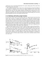
eter choices of the model (6), which are illustrated in Figure 5. For every model, 70
repetitions have been run.
Ŧ5 0 5 10152025
0.00 0.05 0.10
0.15
Two outliers
x

Density
0 5 10 15 20
0.00 0.05 0.10
0.15
Wide noise
x
Density
Ŧ5 0 5 10152025
0.00 0.02 0.04 0.06 0.08
0.10
Noise on one side
x
Density
Ŧ5 0 5 10152025
0.00 0.02 0.04 0.06
0.08 0.10
Noise in between
x
Density
Fig. 5. Simulated models. Note that for the model “2 outliers” the number of points drawn
from the uniform component has been fixedto2.
The misclassification results are given in Table 1. BR-noise yielded the best per-
formance for the “wide noise” model. This is not surprising, because in this model
it’s very likely that the most extreme points on both sides are generated by the uni-
form. With two extreme outliers on one side, it was also optimal. However, it per-
The Noise Component in Model-based Cluster Analysis 137
Table 1. Average misclassification percentages for n = 200
Model/method BR-noise t-mixture improper noise ML-uniform
Two outliers 2.7 7.3 3.9 3.3
Wide noise 8.0 9.6 8.4 9.3

Noise on one side 10.6 8.3 3.6 5.3
Noise in between 8.8 8.7 5.5 7.3
formed much worse in the two models that generated 10% noise at particular places
(“noise on one side” and “noise in between”). The improper noise approach gen-
erally performed very well, almost always better than uniform-ML (which was the
best method for two of the models for n = 500). The t-mixtures-ML didn’t perform
very well, but this is at least partly due to the fact that all simulated models were
of the “normal mixture plus uniform”-type. We will also carry out simulations from
t-mixtures in the future.
6 Conclusion
To deal with noise and outliers in cluster analysis, two new methods have been pro-
posed, which are variants of Banfield and Raftery’s (1993) noise component, namely
the use of an improper density to model the noise and an ML-estimator for a mixture
model including a uniform component. Both methods have some theoretical advan-
tages over BR-noise. Simulations showed a good performance particularly for the
improper noise component with estimated density value. We find the principle to
model outliers and noise by an additional (proper or improper) uniform component
appealing, particularly for cluster analysis applications. It allows a smooth classifi-
cation of points as “noise” or as belonging to a cluster.
Of course it is desirable to apply the ideas to multivariate data as well. This is
possible in a straightforward way for the improper noise approach where k is fixed
in advance by subject matter considerations. Our proposal to estimate k may work as
well for moderate dimensionality, but this is still under investigation.
The ML-uniform approach is problematic in the multivariate setup because of
the large number of potentially reasonable support sets for the uniform distribution.
In principle it could be applied by assuming the support of the uniform component
as rectangular and parallel to the coordinate axes defined by the variables in the data.
The ML solution could then be approximated by the best of several hyperrectan-
gles defined by pairs of data points. It remains to see whether this leads to useful
clusterings.

References
BANFIELD, J. D. and RAFTERY, A. E. (1993): Model-Based Gaussian and Non-Gaussian
Clustering. Biometrics, 49, 803–821.
138 Christian Hennig and Pietro Coretto
CAMPBELL, N. A. (1984): Mixture models and atypical values. Mathematical Geology, 16,
465–477.
CORETTO P. and HENNIG C. (2006): Identifiability for mixtures of distributions from a
location-scale family with uniforms. DISES Working Papers No. 3.186, University of
Salerno.
CORETTO P. and HENNIG C. (2007): Choice of the improper density in robust improper ML
for finite normal mixtures. Submitted.
CUESTA-ALBERTOS, J. A., GORDALIZA, A. and MATRAN, C. (1997): Trimmed k-
means: An Attempt to Robustify Quantizers. Annals of Statistics, 25, 553–576.
DONOHO, D. L. and HUBER, P. J. (1983): The notion of breakdown point. In P. J. Bickel,
K. Doksum, and J. L. Hodges jr. (Eds.): A Festschrift for Erich L. Lehmann, Wadsworth,
Belmont, CA, 157–184.
FRALEY, C. and RAFTERY, A. E. (1998): How Many Clusters? Which Clustering Method?
Answers Via Model Based Cluster Analysis. Computer Journal, 41, 578–588.
HATHAWAY, R. J. (1985): A constrained formulation of maximum-likelihood estimates for
normal mixture distributions. Annals of Statistics, 13, 795–800.
HENNIG, C. (2004): Breakdown points for maximum likelihood-estimators of location-scale
mixtures. Annals of Statistics, 32, 1313–1340.
MCLACHLAN, G. J. and PEEL, D. (2000): Finite Mixture Models, Wiley, New York.
REDNER, R. A. and WALKER, H. F. (1984): Mixture densities, maximum likelihood and the
EM algorithm, SIAM Review, 26, 195–239.
SCHWARZ, G. (1978): Estimating the dimension of a model, Annals of Statistics, 6, 461–464.
Data Mining of an On-line Survey - A Market
Research Application
Karmele Fernández-Aguirre
1

, María I. Landaluce
2
, Ana Martín
1∗
and Juan I.
Modroño
1
1
Universidad del País Vasco (EHU/UPV), Spain

2
Universidad de Burgos (UBU), Spain
Abstract. In this work we apply several data mining techniques that give us deep insight
into knowledge extraction from a marketing survey addressed to the potential buyers of an
university gift shop. The techniques are classified as symmetrical and non-symmetrical. An
advocation for such combination is given as conclusion.
1 Introduction
When a large dataset is obtained from a survey including a large number of questions
it is necessary to extract the information and the relationships inherent to the data in
an ordered and effective way. The data is usually a mixture of subsets of quantitative,
categorical (closed questions) and frecuency (open-ended) questions.
In this work we analyze data extracted from an on-line survey by means of dif-
ferent and complementary methods divided in two categories: symmetrical and non-
symmetrical. The former will be some factor method complemented with classifica-
tion, whereas the latter will comprise some sort of regression models. After present-
ing data and objectives (section 2) we outline methodology and results (section 3)
and finally give some conclusions (section 4).
2 Data and objectives
The University of the Basque Country (UPV/EHU), as part of a large project which
main aim is revamping its corporate image, is about launching a corporate shop (also

considered as a gift or souvenir shop). In order to better know its potential buyers
and the potential success of it, it has set up an online survey to collect information
on its acceptability.
∗
Authors gratefully acknowledge financial support from Grupo de Investigación Consoli-
dado DEC UPV/EHU GIU06/53.
184 Karmele Fernández-Aguirre et al.
Such on-line survey is addressed to the members of the research and teaching
staff, administrative staff and the students of the university. Its main objectives are to
evaluate buying propensity about the corporate products, identify potential buyers’
and non-buyers’ profiles, know desirable characteristics of the products and obtain a
function to be named and considered as a “propensity to buy”.
Table 1 contains the sampling technical characteristics. The access to filling in
the survey was possible only by invitation and there was a period of one month for
doing so. The number of invitations or sample size was fixed per strata and chosen
in order to get a maximum error of 2% of the variability range of the responses for a
95% confidence level. The sampling was thus proportionallly random and the results
were encouraging, with a global response rate of around 40%, though not equally
distributed.
Table 1. Technical characteristics of the on-line survey.
Students Admin. Staff Research & Teaching
Population 48995 1128 3982
Sample size 2289 768 1499
Response (%) 547 (23.9) 444 (57.81) 754 (50.30)
Sampling error 0.042 0.036 0.032
Confidence level 0.95 0.95 0.95
The most relevant questions included in the sample were: a question over general
satisfaction about being a member of the university (5 point scale), a binary question
on general interest about buying the corporate articles, 26 questions on the valuation
(from 1 to 4) of the same number of products (shown in a photo), valuation (from 1

to 7) of 8 proposed desirable characteristics of products (sober, traditional, stylish,
modern, practical, artistic, daring and original) and personal information (gender,
age, post and campus - up to three possible -). We were particularly interested in
getting information on preferences on the products so we intentionally dropped the
middle point in product valuation questions. These questions are those which we
analyze by means of both non-symmetrical and symmetrical methods. We have made
this distinction in order to differentiate between methods that assume some sort of
causality or relationship direction in the variables (i.e., regression methods) and those
who don’t (as factor methods).
3 Methodology and results
3.1 Symmetrical methods: Exploratory multivariate techniques
Depending upon which kind of variables are to be considered as active we can con-
sider a Principal Components (PCA) or a Multiple Correspondence Analysis (MCA),
see
e.g.
, Greenacre (1984), Lebart et al. (1984), Lebart (1994).
Data Mining of an On-line Survey - A Market Research Application 185
PCA of continuous variables and classification
We first consider as active variables the scores given to the question of the desir-
able characteristics of products (original, sober, ), which are measured in a 7 point
scale and may arguably be considered as near-continuous variables. The variables
regarding personal characteristics as gender or age are considered as supplementary
variables, as well as the variables reflecting satisfaction with the institution and the
interest in buying.
The first factor is a size factor which distinguishes between persons who select
higher scores for all or most such characteristics from those who select lower values.
Those who give higher marks are also people who manifest a greater satisfaction,
interest in buying and are over 44 years old. The positive side of the second factor
corresponds to higher scores given to sober, traditional, stylish and artistic and to re-
spondents over 44, teaching-research staff and men and the negative side corresponds

to higher scores given to daring, original and modern. Finally, the third factor locates
individuals scoring high the term practical, who are mostly students and under 30.
After performing a hierarchical clustering on the PCA first 5 axes, using the gen-
eralized Ward criterion, this results in three clusters. The first one (46%) corresponds
exactly to those on the positive side of the first factor (over 44, fully satisfied, with
buying interest, high scores to all characteristics). The second one (31%) to individ-
uals who rank high the characteristics of original, daring, modern and practical and
who are students, under 30, neither satisfied or dissatisfied and who do not manifest
buying interest. This is a group who might be attracted to the first group, composed
of feasible buyers, by improving the characteristics of the products in the way they
consider important. The last cluster (23%) give low scores to most of the characteris-
tics and manifest no interest in buying and are also indifferent to the institution. This
group seems a difficult one to reach to.
This first analysis provides three main directions of variability by means of a
PCA. The clustering over the main factors helps to group individuals into homoge-
neous families where each cluster represents a market segment with different char-
acteristics and reachable through different marketing strategies or perhaps products
not considered here.
MCA of categorical variables and classification
As a second factor method, we choose the categorical variables referring to valuation
of the 26 articles (after seeing a displayed photo) in a scale 1-4 as the active variables
of a MCA. As supplementary variables we choose the products characteristics, the
satisfaction variable, the intention to buy and the individuals’ personal data.
Figure 1 shows the projection of the active categories on the MCA main plane.
It shows how the first factor represents a global propensity to buy, roughly ordering
categories from left to right with respect to their probability to buy, from lower to
higher. The plane shows a typical Guttman effect with the second factor reflecting
differences between extreme and centered opinions.
186 Karmele Fernández-Aguirre et al.
Factor 1 - 14.13 %

Factor 2 - 6.67 %
Umbre=1
Umbre=2
Umbre=3
Umbre=4
Keyri=1
Keyri=2
Keyri=3
Keyri=4
Tie=1
Tie=2
Tie=3
Tie=4
Hat=1
Hat=2
Hat=3
Hat=4
Kerf1=1
Kerf1=2
Kerf1=3
Kerf1=4
Kerf2=1
Kerf2=2
Kerf2=3
Kerf2=4
Trayp=1
Trayp=2
Trayp=3
Trayp=4
Trays=1

Trays=2
Trays=3
Trays=4
T-shi=1
T-shi=2
T-shi=3
T-shi=4
Fem-T=1
Fem-T=2
Fem-T=3
Fem-T=4
Sweat=1
Sweat=2
Sweat=3
Sweat=4
Cap=1
Cap=2
Cap=3
Cap=4
Light=1
Light=2
Light=3
Light=4
Pin=1
Pin=2
Pin=3
Pin=4
SkinW=1
SkinW=2
SkinW=3

SkinW=4
MetWa=1
MetWa=2
MetWa=3
MetWa=4
Walle=1
Walle=2
Walle=3
Walle=4
Backp=1
Backp=2
Backp=3
Backp=4
Bag=1
Bag=2
Bag=3
Bag=4
BlueP=1
BlueP=2
BlueP=3
BlueP=4
Black=1
Black=2
Black=3
Black=4
Silve=1
Silve=2
Silve=3
Silve=4
SWBPe=1

SWBPe=2
SWBPe=3
SWBPe=4
Cup=1
Cup=2
Cup=3
Cup=4
Mouse=1
Mouse=2
Mouse=3
Mouse=4
Sculp=1
Sculp=2
Sculp=3
Sculp=4
Fig. 1. MCA: active categories on plane (1,2).
With respect to the projections of the supplementary categories, it is shown in
Figure 2 that the first factor is positively related to the satisfaction with the institution
and the declared propensity to buy. This shows the relationship of these variables
with the overall propensity to buy individually the 26 products.
Factor 1 - 14.13 %
Factor 2 - 6.67 %
Satis=1
Satis=2
Satis=3
Satis=4
Satis=5
BuyLo=1
BuyLo=2
Satis

Fig. 2. MCA: supplementary categories on plane (1,2).
A mixed classification in three steps is carried out on 8 MCA first principal axes.
This process starts by choosing a partition in 10 clusters with random initial centers
and then update those centers calculating the centroids of the groups of individuals
nearest to the centers (K-means algorithm); the process is repeated until the clusters
are stable. We reduce further the number of clusters by means of a hierarchical algo-
rithm (generalized Ward’s method) and refine the resulting partition with a consol-
Data Mining of an On-line Survey - A Market Research Application 187
idation step with re-assignment (testing moving centers with convergence achieved
in 7 iterations). This results in a partition of 6 classes with an inter inertia over total
inertia ratio of 55.62%. The positions of the final centers on the plane are given in
Figure 3, and are following the pattern set by the active categories on this same plane.
Factor 1 - 14.13 %
Factor 2 - 6.67 %
Cluster 1 / 6
Cluster 2 / 6
Cluster 3 / 6
Cluster 4 / 6
Cluster 5 / 6
Cluster 6 / 6
Fig. 3. Classification on MCA factors. Clusters centers and relative sizes represented by circle
diameters.
The partition description is as follows. Cluster 1 (15.73%) contains those who
would prior buy, say is very likely to buy for many products, are over 44, fully satis-
fied, females, members of the teaching and research staff, give high scores to stylish
and traditional. Cluster 2 (17.91%) is formed by those who are likely to buy, over 44,
would prior buy and rank highly stylish, traditional and sober. In cluster 3 (17.74%)
predominate those who say it is unlikely to buy sober and stylish products (metal-
lic) but it is likely to buy original, modern and practical products (textiles and bags).
Cluster 4 (12.80%) groups individuals unlikely to buy anything with low scores for

stylish products. Cluster 5 (18.66%) is composed of individuals very unlikely to buy,
aged between 18 and 22, students, from Gipuzkoa campus, neither satisfied or dis-
satisfied and with low scores on traditional, sober or stylish. Finally, on cluster 6
(17.16%) are those who are very unlikely to buy, between 30 and 44, males and with
low marks for all characteristics of the products.
This MCA confirms the tight relationship between the interest to buy articles
featuring the logo (before visualization), the degree of satisfaction about the insti-
tution and the scores given to the proposed desirable characteristics of the products.
The clustering process shows marketing implications on the buyers’ and non-buyers’
personal characteristics and on which articles are perceived as stylish, traditional and
sober and which ones as modern, original and practical. Furthermore, the parabolic
path apperaring in Figure 1 is similar to those shown in Figures 2 and 3, reinforcing
its interpretation as an indicator of the propensity to buy the displayed products.
188 Karmele Fernández-Aguirre et al.
3.2 Non-symmetrical methods: regression related techniques
In this section we consider methods where one variable is chosen to be depending on
others. In this work, the variable of interest is the probability, or propension, to buy
and is exactly our choice for the endogeneous variable.
PLS path modelling
PLS path modelling (see,
e.g.
, Tenenhaus et al. (2005)) is a technique based on the re-
lationships between latent variables in a regression framework where such variables
are constructed with underlying manifest variables (MV). In this case, the variables
are those obtained with the questions of the survey.
We are going to construct a global propensity to buy using all manifest variables,
resulting in a global latent variable (LV). At the same time, we want unidimensional
partial propensities to buy groups of products and these to be autoselected by the
data, we do not want to impose any additional structure, other than the imposed by
the model itself. These will also have the form of LVs and will be sought with a

previous PCA of the valuations of all the 26 products displayed in the survey.
Table 2 contains the 8 groups of products formed in the way explained above.
These groupings originate directly 8 partial LVs, using mode B.
Table 2. Groups of products to be considered as LV.
label LV products
umbh [
1
umbrella, hat
tie [
2
tie, kerchief no.1, kerchief no.2
textiles [
3
T-shirt, T-shirt-V, sweater, cap
bag [
4
plastic tray, leather tray, backpack, bag, cup
wat [
5
leather-strapped watch, metallic-strapped watch, wallet
mous [
6
keyring, lighter, mousepad
scul [
7
pin, sculpture
pens [
8
blue pen, black pen, silver pen, silver pen in wooden case
Selecting all products valuations, we construct the global propensity to buy using

mode A. Finally, we formulate the external model [ =

8
j=1
E
j
[
j
+ Q.
Figure 4 shows the path model specified. The numbers are correlations and show
relatively high values between the partial LVs and the global one. We can also see
the pairwise correlations between individual MVs and the LVs.
The actual estimates of the external model parameters are given in equation (1).
These show higher values for textiles, bags and pens products groups, which are
those with a higher acceptability among the respondents.
E([)=0.0865 ∗umbh+ 0.1335∗tie+ 0.2041∗textiles+ 0.2114∗bag
+0.1791∗wat + 0.1292∗mous+ 0.0881∗scul+ 0.2322∗pens
(1)
Data Mining of an On-line Survey - A Market Research Application 189
Umbrella
Hat
Tie
Kerchief1
TŦshirt
Sweater
Trayplas
Backpack
Bag
Cup
WatchMet

Wallet
Keyring
Lighter
Mousepad
Pin
Sculpture
Pen Blue
Pen Black
Pen Silver
Pen S. w/ case
[
[
Tie
1
2
[
3
4
[
5
6
[
7
[
[
8
Hat
Umbrella
Kerchief1
Kerchief2

TŦshirt
TŦshirtŦV
Sweater
Cap
Trayplas
Backpack
Bag
Cup
WatchMet
Wallet
Keyring
Lighter
Mousepad
Pin
Sculpture
Pen Blue
PenBlack
Pen Silver
Pen S. w/ case
0.84
0.68
0.82
0.84
0.83
0.68
0.72
0.88
0.91
0.85
0.85

0.68
0.78
0.77
0.72
0.89
0.66
0.96
0.66
0.93
0.90
0.73
0.87
0.88
0.83
0.78
0.64
0.86
0.78
[
0.79
0.89
0.91
0.48
0.57
0.49
0.60
0.62
0.71
0.71
0.64

0.69
0.58
0.67
0.66
0.65
0.61
0.74
0.75
0.72
0.69
0.58
0.53
0.65
0.45
0.70
0.76
0.75
0.73
umbh
tie
textiles
bag
wat
mous
scul
pens
0.85
WatchLeather
Trayleather
WatchLeather

Kerchief2
TŦshirtŦV
Cap
Trayleather
0.75
[
Fig. 4. PLS path diagram for products to be sold at the university shop.
In order to get a potential buyers’ characterization (similar to the projection of
supplementary variables in a factor analysis), we perform a regression on the de-
sirable characteristics of the products and the respondents’ personal characteristics.
This is actually a Principal Components Regression (PCR), since the desirable char-
acteristics are highly correlated, selecting 2 main components out of the 7 original
variables.
E([)=−0.85 + 0.07 ∗F1 (orig., daring, practical, artistic, modern)
+0.11∗F2 (traditional, sober, stylish)−0.25∗male
+0.15∗satisfied +0.26 ∗very satisfied+ 0.07∗age(+44)
+0.06∗teaching-research staff−0.10∗higher education
+1.18∗overall propensity to buy a logo product
+0.14∗campus: Araba +0.12 ∗campus: Bizkaia
R
2
= 0.4848
All parameters whose estimates are shown are significant at the 5% level, both
using bootstrap confidence intervals and usual t-test statistics. These estimates show
how those individuals most satisfied with the university are more likely to buy, along
with women. It is also so for those who have a prior intention to buy, members of
teaching and research staff, older age and those proceeding from the campuses of
Bizkaia and Araba from over those from Gipuzkoa. With respect to product charac-
teristics, those marking as more important the terms traditional, sober and stylish are
more likely to buy than individuals giving more importance to aspects as modern,

practical and so on.
190 Karmele Fernández-Aguirre et al.
Logit models
Finally, we have calculated a logit regression (see,
e.g.
, Hosmer and Lemeshow
(2000)) on individuals’ personal characteristics, products characteristics and the sat-
isfaction variable where the dichotomous endogeneus variable is the response (yes
or no) to the question if the respondent would, in general, buy university corporate
products. This is a prior probability in the sense that individuals had to respond to
that question before actually seeing the products.
We have also considered the construction of a posterior probability to buy and
then estimated another logit model with this probability as the endogeneous vari-
able. Thus, an individual is considered to be likely to buy one product if he or she
scores 3 (likely) or 4 (very likely) for that product. In the same way, an individual is
considered to buy articles if he or she would likely buy more than 25% of all articles
(at least 7 articles).
As in the PLS path model case, the desirable characteristics of the products are
highly correlated and we have substituted them by two principal PCA factors (after
performing a Varimax rotation).
We end up with the following two model estimates:
1. Prior probability model estimates (Nagelkerke R
2
= 0.140):
X

E = −0.510 + 0.267 ∗teach./res. + 0.307∗Bizkaia+ 0.398∗age over 44
+0.797∗satisfied +1.160 ∗very satisfied+
+0.220∗F1 (innovative+practical)+ 0.272∗F2 (classic)
2. Posterior estimates (Nagelkerke R

2
= 0.502):
X

E = −1.298 + 0.537 ∗student + 0.584∗teach./res.−0.794∗male
+0.367∗satisfied +0.710 ∗very satisfied+ 0.339 ∗F2 (classic)
+2.979∗buying initial interest
The prior probability model yields very similar results to those from the PLS path
model and the factor analyses performed in the previous subsection. The posterior
probability model yields, with a better fit, results not so similar, what can be due to
the particular construction of the endogeneous variable. That construction is sensitive
but also subjective and it can only be considered as a help to better know the structure
of the data.
4 Conclusions
Each different technique used shows specific, though related, conclusions given its
different objectives. The symmetrical methods (PCA, MCA) combined with Cluster
Analysis help to learn what is contained in the data, including relationships and clas-
sifications of similar individuals. On the other hand, non-symmetrical methods as
Data Mining of an On-line Survey - A Market Research Application 191
PLS or Logit regressions allow for modelling individuals’ global and partial (group)
behaviour using inference tools to select a better model with a good fit to the data.
The methods exposed above extract consistently some facts from this particular
data. The gift shop potential buyers’ general characteristics become clear (satisfied
with the institution, members of the teaching-research staff, women ). At the same
time, it is also clear the general characteristics of the articles shown (traditional, )
and the sort of characteristics of possible successful articles not covered in current
product line (practical, original or modern). It seems that a better, more modern,
design is needed to reach other market segments.
The marketing implications obtained have been somewhat conditioned upon the
actual articles displayed with photographs in the on-line questionnaire. It has been

observed that many have been perceived as stylish and traditional (generally of a
metallic aspect) and of little appeal for the young. As a general issue, this work rec-
ommends the promotion of articles with the characteristics mentioned above and,
particularly, belonging to the groups of textiles, bags and desktop articles which
would yield a better acceptance for this target public in the opening university gift
shop.
All in one, it can be said that these data mining techniques yield useful directions
for the university marketing policy, regarding the corporate shop. The combination
of techniques, though never fully exhaustive, reinforces the confidence on the results
as it is improbable to having missed important patterns in the data.
References
GREENACRE, M. (1984): Theory and Applications of Correspondence Analysis. (Academic
Press, London)
HOSMER, D. R. and LEMESHOW, S. (2000): Applied Logistic Regression. 2nd Edition, Wi-
ley & Sons Inc, USA
LEBART, L. (1994): Complementary use of correspondence analysis and cluster analysis. In:
Greenacre, M.J. and Blasius, J. (Eds.): Correspondence Analysis in the Social Sciences.
LEBART, L., MORINEAU, A. and WARWICK, K. (1984): Multivariate Descriptive Statisti-
cal Analysis. (Wiley, NewYork)
TENENHAUS, M., E. VINZI, V., CHATELIN, Y.M. and LAURO, C. (2005): PLS path mod-
eling. Computational Statistics & Data Analysis, 48, 159–205.
Factorial Analysis of a Set of Contingency Tables
Amaya Zárraga and Beatriz Goitisolo
Departamento de Economía Aplicada III, UPV/EHU, Bilbao, Spain
{amaya.zarraga, beatriz.goitisolo}@ehu.es
Abstract. The aim of this work is to present a method of joint factorial analysis of several
contingency tables. This method that we have called Simultaneous Analysis (SA), is especially
appropriate to analyze frequency tables whose row margins are different, for example when
the tables are from different samples or different time points. Furthermore, SA may be applied
to the joint analysis of more than two data tables in which rows refer to the same entities, but

columns may be different.
SA allows us to maintain the structure of each table in the overall analysis by centering
each table internally with its margins, as is done in Correspondence Analysis (CA) and pro-
vides a joint description of the different structures contained within each table. Besides jointly
studying the intrastructure of the tables, SA permits an overall comparison of the similarities
and differences between the tables.
1 Introduction
The need of jointly analyzing several contingency tables has produced several facto-
rial methods.
Some of the proposed methods consist in the analysis of the table obtained as
sum of the separated contingency tables and/or the analysis of the table obtained as
juxtaposition of the initial tables (Cazes (1980) and (1981)) and the Intra Analysis
(Escofier (1983)). Nevertheless, in Zárraga and Goitisolo (2002) it is shown that there
are situations where none of these methods permits an analysis of the similarities
among rows that mantains the similarity in the analyses of the separated tables.
The aim of this work is to present a factorial method for the joint analysis of sev-
eral contingency tables that allows, in a similar way to correspondence analysis, the
study of the similarity among the set of rows, of columns and the relations between
both sets.
Also cite the non symmetrical analysis (D’ Ambra and Lauro (1984) and Lauro
and D’ Ambra (1989)) and more recently the Multiple Factor Analysis for Contin-
gency Tables (Pagès and Bécue-Bertaut (2006)).
220 Amaya Zárraga and Beatriz Goitisolo
2 Methodology
Let T = {1, ,t, ,T} be the set of contingency tables to be analyzed. Each of
them classifies the answers of n
t
individuals with respect to two categorical vari-
ables. All the tables have one of the variables in common, in this case the row vari-
able with categories I = {1, ,i, ,I}. The other variable of each contingency table

can be different or the same variable observed at different time points or in different
subsamples. On concatenating all these contingency tables, a joint set of columns
J = {1, , j, ,J} is obtained. The element n
ijt
corresponds to the total number of
individuals who choose simultaneously the categories i ∈I of the first variable and
j ∈ J
t
of the second variable, for table t ∈T. Sums are denoted in the usual way, for
example, n
i.t
=

j∈J
t
n
ijt
,andn denotes the grand total of all T tables.
In order to maintain the internal structure of each table t, SA begins by obtaining
the relative frequencies of each table as usually done in CA: p
t
ij
= n
ijt
/n
t
so that

i∈I


j∈J
t
p
t
ij
= 1 for each table t. It is important to keep in mind that these relative
frequencies are different from those obtained when calculating the relative frequency
for the whole matrix: p
ijt
= n
ijt
/n.
The method that we propose is carried out in three stages.
2.1 Stage one: CA of each contingency table
Since in SA it is important for each table to maintain its own structure, the first
stage carries out a classical CA of each of the T contingency tables. These separate
analyses also allow us to check for the existence of structures common to the different
tables. From these analyses it is possible to obtain the weighting used in the next
stage.
CA on the t-th contingency table can be carried out by calculating the singular
value decomposition (SVD) of the matrix X
t
, whose general term is:

p
t
i.

p
t

ij
−p
t
i.
p
t
. j
p
t
i.
p
t
. j


p
t
. j
Let D
t
r
and D
t
c
be the diagonal matrices whose diagonal entries are respectively the
marginal row frequencies p
t
i.
and column frequencies p
t

. j
. From the SVD of each
table X
t
we retain the first squared singular value (or eigenvalue, or principal inertia),
denoted by O
t
1
.
2.2 Stage two: analysis of intrastructure
In the second stage, in order to balance the influence of each table in the joint analy-
sis, measured by the inertia, and to prevent this joint analysis from being dominated
by a particular table, SA will include a weighting on each table, D
t
. With this aim, in
SA, D
t
= 1/O
t
1
, where O
t
1
denotes the first eigenvalue (square of first singular value)
of the separate CA of table t (stage one). This weight is similar to the one used in
Multiple Factor Analysis (MFA) (Escofier and Pagès (1988)).