Data Analysis Machine Learning and Applications Episode 1 Part 9 doc

Factorial Analysis of a Set of Contingency Tables 221
As a result, SA proceeds by performing a principal component analysis (PCA)
of the matrix X, X =

√
D
1
X
1

√
D
t
X
t

√
D
T
X
T

The PCA results are also obtained using the SVD of X, giving singular values
√
O
s
on the s-th dimension and corresponding left and right singular vectors u
s
and
v
s

.
We calculate projections on the s-th axis of the columns as principal coordinates
g
s
, g
s
= O
s
D
−1/2
c
v
s
where D
c
(J ×J), is a diagonal matrix of all the column masses,
that is all the D
t
c
.
One of the aims of the joint analysis of several data tables is to compare them
through the points corresponding to the same row in the different tables. These points
will be called partial rows and denoted by i
t
.
The projection on the s-th axis of each partial row is denoted by f
t
is
and the vector
of projections of all the partial rows for table t is denoted by f

t
s
, f
t
s
=
(D
t
r
)
−1/2
[0
√
D
t
X
t
0] v
s
Especially when the number of tables is large, comparison of partial rows is
complicated. Therefore each partial row will be compared with the (overall) row,
projected as f
s
=(D
w
)
−1

√
D

1
X
1

√
D
t
X
t

√
D
T
X
T

v
s
=(D
w
)
−1
X v
s
where
D
w
is the diagonal matrix whose general term is

t∈T


p
t
i.
. The choice of this matrix
D
w
allows us to expand the projections of the (overall) rows to keep them inside the
corresponding set of projections of partial rows, and is appropriate when the partial
rows have different weights in the tables. With this weighting the projections of the
overall and partial rows are related as follows:
f
is
=

t∈T
√
p
t
i.

t∈T
√
p
t
i.
f
t
is
So the projection of a row is a weighted average of the projections of partial rows. It

is closer to those partial rows that are more similar to the overall row in terms of the
relation expressed by the axis and have a greater weight than the rest of the partial
rows. The dispersal of the projections of the partial rows with regard to the projection
of their (overall) row indicates discrepancies between the same row in the different
tables.
Notice that if p
t
i.
is equal in all the tables then f
s
=(1/T)

t∈T
f
t
s
, that is the
overall row is projected as the average of the projections of the partial rows.
Interpretation rules for simultaneous analysis
In SA the transition relations between projections of different points create a simul-
taneous representation that provides more detailed knowledge of the matter being
studied.
Relation between f
t
is
and g
js
: The projection of a partial row on axis s depends
on the projections of the columns:
f

t
is
=
√
D
t
√
O
s

j∈J
t
p
t
ij
p
t
i.
g
js
222 Amaya Zárraga and Beatriz Goitisolo
Except for the factor

D
t
/O
s
, the projection of a partial row on axis s, is, as in CA,
the centroid of the projections of the columns of table t.
Relation between f

is
and g
js
: The projection of an overall row on axis s may be
expressed in terms of the projections of the columns as follows:
f
is
=

t∈T
√
D
t
√
p
t
i.

t∈T

p
t
i.

1
√
O
s

j∈J

t
p
t
ij
p
t
i.
g
js

The projection of the row is therefore, except for the coefficients

D
t
/O
s
, the
weighted average of the centroids of the projections of the columns for each table.
Relation between g
js
and f
is
or f
t
is
: The projection on the axis s, of the column j
for table t, can be expressed in the following way:
g
js
=

√
D
t
O
s


i∈I


t∈T

p
t
i.


p
t
i.

p
t
ij
−p
t
i.
p
t
. j

p
t
i.
p
t
. j

f
is

This expression shows that the projection of a column is placed on the side of
the projections of the rows with which it is associated, compared to the hypothesis
of independence, and on the opposite side of the projections of those to which it is
less associated.
This projection is, according to partial rows:
g
js
=

D
t
O
s


i∈I

p
t
i.


p
t
ij
−p
t
i.
p
t
. j
p
t
i.
p
t
. j



t∈T

p
t
i.
f
t
is


The same aids to interpretation are available in SA as in standard factorial anal-

ysis as regards the contribution of points to principal axes and the quality of display
of a point on axis s.
2.3 Stage three: comparison of the tables: interstructure
In order to compare the different tables, SA allows us, to represent each of them by
means of a point and to project them on the axes.
The coordinate of table t on axis s, f
ts
, represents the projected inertia of the table
on the axis and, therefore, indicates the importance of the table in the determination
of the axis. Thus, f
ts
=

j∈J
t
p
t
. j
g
2
js
= Inertia
s
(t) where Inertia
s
(t) represents the
projected inertia of the sum of columns of the table t on the axis s.
Due to the weighting of the tables chosen by SA, the maximum value of this
inertia on the firstaxisis1.Avalueof f
ts

close to 0 would indicate orthogonality
between the first axes of the separate analyses with regard the Simultaneous Anal-
ysis. A value of f
ts
close to 1 would indicate that the axis of the joint analysis is
approximately the same as in the separate analysis of each table. So, if all the tables
present a coordinate close to the maximum value, 1, on the first factorial axis of the
SA, the projected inertia onto it is approximately T, the number of tables, and this
confirms that this first direction is accurately depicting the relevant associations of
each table.
Factorial Analysis of a Set of Contingency Tables 223
2.4 Relations between factors of the analyses
In SA it is also possible to calculate the following measurements of the relation
between the factors of the different analyses.
Relation between factors of the individual analyses: The correlation coefficient
can be used to measure the degree of similarity between the factors of the separate
CA of different tables. This is possible when the marginals p
t
i.
are equal.
When p
t
i.
are not equal, Cazes (1982) proposes calculating the correlation coef-
ficient between factors, assigning weight to the rows corresponding to the margins
of one of the tables. Therefore, these weights, and the correlation coefficient as well,
depend on the choice of this reference table. In consequence, we propose to solve this
problem of the weight by extending the concept of generalized covariance (Méot and
Leclerc (1997)) to that of generalized correlation (Zárraga and Goitisolo (2003)).
The relation between the factors s and s


of the tables t and t

respectively would
be calculated as:
r(f
st
,f
s

t

)=

i∈I
f
ist
√
O
t
s

p
t
i.

p
t

i.

f
is

t


O
t

s

where f
ist
and f
is

t

are the projections on the axes s and s

of the separate CA of
the tables t and t

respectively and where O
t
s
and O
t

s


are the inertias associated with
these axes. This measurement allows us to verify whether the factors of the separate
analyses are similar and check the possible rotations that occur.
Relation between factors of the SA and factors of the separate analyses: Like-
wise, it is possible to calculate for each factor s of the SA, the relation with each of
the factors s

of the separate analyses of the different tables:
r(f
s

t
,f
s
)=

i∈I
f
is

t

O
t
s


p
t

i.


t∈T

p
t
i.

f
is
√
O
s
If all the tables of frequencies analysed have the same row weights this measure-
ment is reduced to:
r(f
s

t
,f
s
)=

i∈I
p
t
i.
f
is


t
f
is


i∈I
p
t
i.
(
f
is

t
)
2


i∈I
p
t
i.
( f
is
)
2
that is, the classical correlation coefficient between the factors of the separate analy-
ses and the factors of SA.
3 Application

In this section we apply SA to the data taken from an on-line survey drawn up by the
Spanish Ministry of Education and Science, from January to March 2006, to Spanish
students who participate in the Erasmus program in European universities.
This application presents a comparative study for Spanish students, according to
gender, of the relationships between the countries that they choose as destination to
carry out the university interchange in the Erasmus program and the scientific fields
in which they are studying.
224 Amaya Zárraga and Beatriz Goitisolo
The 15 countries that they choose as destination are Austria, Belgium, Czech
Republic, Denmark, Finland, France, Germany, Ireland, Italy, Netherlands, Norway,
Poland, Portugal, Sweden and United Kingdom. The scientific fields in which they
are studying are: Social and Legal Sciences, Engineering and Technology, Humani-
ties, Health Science and Experimental Science.
Therefore, we have two data tables whose rows (countries) and columns (sci-
entific fields) correspond to the same modalities but refer to two different sets of
individuals, depending on their gender. In these tables both the marginals and the
grand-totals are different. This fact suggests analyzing the tables by SA since the re-
sults of applying other methods can be affected by the above mentioned differences
(Zárraga and Goitisolo (2002)).
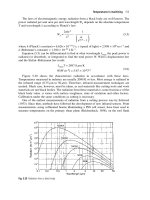
The first factorial plane of SA (figure 1) explains nearly 60% of total inertia. In
the plane we observe that male and female students of Humanities Area, Health Sci-
ence and specially Engineering and Technology have a similar behavior in the choice
of the country of destination to realize their studies, whereas students of Social and
Legal Sciences and of Experimental Science choose different countries as destiny
depending on their gender.
The plane shows that students of Humanities Area, both male and female, choose
the United Kingdom as destiny country, followed by Ireland. The countries chosen
as destiny for students of both gender of Engineering and Technology are mainly
Austria, Sweden and Denmark. Finally, the males and females students of Health
Science Area prefer Portugal and Finland.

The students of Experimental Science Area select different countries to realize
the interchange depending on their gender. While male students go mainly to Portu-
gal and Netherlands, females go to Norway.
Also students of Social and Legal Sciences Area have a different behavior. The
Netherlands and Ireland are selected as destiny country by males and females but
males also go to Belgium, the United Kingdom and Italy while females do it to
Norway and Sweden.
The projection of partial rows of each table, joined by segments, allows us to
appreciate the differences between males and females in each destiny country. We
will only remark some of them.
For example, United Kingdom is a country to which males and females students
go in a greater proportion among the students of Humanities. Nevertheless males
also choose United Kingdom to carry out Social and Legal studies whereas females
do not.
Male and female students that come to Portugal agree in selecting this country
over the average for Health degrees. But, males also go to Portugal to study Ex-
perimental Science while females prefer this country for studies of Engineering and
Technology.
Spanish students who go to Finland share the selection of this country over the
rest of the countries to study in the areas of Health and Engineering but there are
more females in the former area and males in the last one.
Factorial Analysis of a Set of Contingency Tables 225
Fig. 1. Projection of columns, overall rows and partial rows
In the other hand, not big differences between males and females are found in
Germany, France, Belgium and Norway as it is indicate by the close projections of
overall and partial rows.
As conclusion of this application we can say that Simultaneous Analysis allows
us to show the common structure inside each table as well as the differences in the
structure of both tables. A more extensive application to the joint study of the inter
and intra-structure of a bigger number of contingency tables can be found in Zárraga

and Goitisolo (2006).
4 Discussion
The joint study of several data tables has given rise to an extensive list of factorial
methods, some of which have been gathered by Cazes (2004), for both quantitative
and categorical data tables. In the correspondence analysis (CA) approach Cazes
shows the similarity between some methods in the case of proportional row mar-
gins and shows the problem that arises in a joint analysis when the row margins are
different or not proportional.
Comments on the appropriateness of SA and a comparison with different meth-
ods, especially with Multiple Factor Analysis for Contingency Tables (Pagès and
Bécue-Bertaut (2006)), in the cases where row margins are equal, proportional and
not proportional between the tables can be found in Zárraga and Goitisolo (2006).
226 Amaya Zárraga and Beatriz Goitisolo
5 Software notes
Software for performing Simultaneous Analysis, written in S-Plus 2000 can be found
in Goitisolo (2002). The AnSimult package for R can be obtained from the authors.
References
CAZES, P. (1980): L’ analyse de certains tableaux rectangulaires décomposés en blocs:
généralisation des propriétes rencontrées dans l’ étude des correspondances multiples. I.
Définitions et applications à l’ analyse canonique des variables qualitatives. Les Cahiers
de l’ Analyse des Données, V, 2, 145–161.
CAZES, P.(1981): L’ analyse de certains tableaux rectangulaires décomposés en blocs:
généralisation des propriétes rencontrées dans l’ étude des correspondances multiples.
IV. Cas modèles. Les Cahiers de l’ Analyse des Données, VI, 2, 135–143.
CAZES, P. (1982): Note sur les éléments supplémentaires en analyse des correspondances II.
Tableaux multiples. Les Cahiers de l’ Analyse des Données, VII, 133–154.
CAZES, P. (2004): Quelques methodes d’ analyse factorielle d’ une serie de tableaux de don-
nées. La Revue de Modulad, 31, 1–31.
D’ AMBRA, L. and LAURO, N. (1989): Non symetrical analysis of three-way contingency
tables. Multiway Data Analysis, 301–315.

ESCOFIER, B. (1983): Généralisation de l’ analyse des correspondances à la comparaison de
tableaux de fréquence. INRIA, Mai, 207, 1–33.
ESCOFIER, B and PAGÈS, J. (1988 (1998, 3e édition) ): Analyses Factorielles Simples et
Multiples. Objetifs, méthodes et interprétation. Dunod, París.
GOITISOLO, B. (2002): El análisis simultáneo. Propuesta y aplicación de un nuevo método
de análisis factorial de tablas de contingencia. Phd Thesis. Basque Country University
Press. Bilbao. Spain.
LAURO, N. and D’ AMBRA, L. (1984): L’ Analyse non symétrique des correspondances.
Data Analysis and Informatics, III, 433–446.
MÉOT, A. and LECLERC, B. (1997): Voisinages a priori et analyses factorielles: Illustration
dans le cas de proximités géographiques. Revue de Statistique Appliquée, XLV, 25–44.
PAGÈS, J. and BÉCUE-BERTAUT, M. (2006): Multiple Factor Analysis for Contingency
Tables. In: M. Greenacre and J.Blasius (Eds.): Multiple Correspondence Analysis and
Related Methods. Chapman & Hall/CRC, 299–326.
ZÁRRAGA, A. and GOITISOLO, B. (2002): Méthode factorielle pour l’analyse simultanée
de tableaux de contingence. Revue de Statistique Appliquée L(2), 47-70.
ZÁRRAGA, A. and GOITISOLO, B. (2003): Étude de la structure Inter-tableaux à travers
l’Analyse Simultanée. Revue de Statistique Appliquée LI(3), 39-60.
ZÁRRAGA, A. and GOITISOLO, B. (2006): Simultaneous Analysis: A Joint Study of Sev-
eral Contingency Tables with Different Margins. In: M. Greenacre and J.Blasius (Eds.):
Multiple Correspondence Analysis and Related Methods. Chapman & Hall/CRC, 327–
350.
Non Parametric Control Chart by Multivariate
Additive Partial Least Squares via Spline
Rosaria Lombardo
1
, Amalia Vanacore
2
and Jean-Francçois Durand
3

1
Faculty of Economics, Second University of Naples, Italy

2
Faculty of Engineering, University of Naples “Federico II", Italy

3
Faculty of Maths, University of Montpelier II, France

Abstract. Statistical process control (SPC) chart is aimed at monitoring a process over time in
order to detect any special event that may occur and find assignable causes for it. Controlling
both product quality variables and process variables is a complex problem. Multivariate meth-
ods permit to treat all the data simultaneously extracting information on the “directionality"
of the process variation. Highlighting the dependence relationships between process variables
and product quality variables, we propose the construction of a non-parametric chart, based on
Multivariate Additive Partial Least Squares Splines; proper control limits are built by applying
the Bootstrap approach.
1 Introduction
The multivariate nature of product quality (response or output variables) and pro-
cess characteristics (predictors or input variables) highlights the limits of any anal-
ysis based exclusively on descriptive and univariate statistics. On the other hand,
the possibility for process managers of extracting knowledge from large databases,
opens the way to analyze the multivariate dependence relationships between qual-
ity product and process variables via predictive and regressive techniques like PLS
(Tenenhaus, 1998; Wold, 1966) and its generalizations (Durand, 2001; Lombardo et
al., 2007). In this paper, the application of a multivariate control chart based on a
generalization of PLS-T
2
chart (Kourti and MacGregor, 1996) is proposed in order
to analyze the in-control process and monitoring it over time. Furthermore, in order

to face the problem of the unknown distribution of the statistic to be charted, a non-
parametric approach is applied for the selection of the control limits. Distribution-
free or non-parametric control charts have been proposed in literature to overcome
the problems related to the lack of normality in process data. An overview in lit-
erature on univariate non-parametric control charts is given by Chakraborti et al.
(2001). The principles on which non-parametric control charts rest can be general-
ized to multivariate settings. In particular, the bootstrap approach to estimate control
202 Rosaria Lombardo, Amalia Vanacore and Jean-Francçois Durand
limits (Wu and Wang, 1997; Jones and Woodall, 1998; Liu and Tang, 1996) has been
followed.
2 Multivariate control charts based on projection methods
A standard multivariate quality control problem occurs when an observed vector of
measurements on quality characteristics exhibits a significant shift from a set of tar-
get (or standard) values. The first attempt to face the problem of multivariate process
control is due to Hotelling (1947) who introduced the well-known T
2
chart based
on variance-covariance matrix. Successively, different approaches to take into ac-
count the multivariate nature of the problem were proposed (Woodall, Ncube, 1985;
Lowry et al., 1992; Jackson, 1991; Liu, 1995; Kourti and MacGregor, 1996, Mac-
Gregor, 1997). In particular, we focus on the approach based on PLS components
proposed by Kourti and MacGregor (1996), in order to monitor over time the depen-
dence structure between a set of process variables and one or more product quality
variables (Hawkins, 1991). The PLS approach proves to be effective in presence of
a low-ratio of observations to variables and in case of multicollinearity among the
predictors, but a major limit of this approach is that it assumes a linear dependence
structure. Generally, linearity assumption in a model is reasonable as first research
step, but in practice relationships between the process variables and the product qual-
ity variables are often non-linear and in order to study the dependence structure it
could be much more appropriate the use of non-linear models (PLS via Spline, i.e.

PLSS; Durand, 2001) as proposed by Vanacore and Lombardo (2005). The PLSS-T
2
chart allows to handle non-linear dependence relationships in data structure, miss-
ing values and outliers, but it presents two major drawbacks: 1) it does not take into
account the possible effect of interactions between process variables; 2) it requires
testing normality assumption on the component scores, even when original data are
multinormal (in fact, in case of spline, i.e. non linear transformations of original
process variables, the multinormality assumption cannot be guaranteed anymore).
To overcome these drawbacks we present non-parametric Multivariate Additive PLS
Spline-T
2
chart based on Multivariate Additive PLSS (MAPLSS, Lombardo et al.,
2007) briefly described in sub-section 2.2.
2.1 Review of MAPLSS
MAPLSS is just the application of linear PLS regression of the response (matrix Y
of dimension n,q) on linear combinations of the transformed predictors (matrix X
of dimension n, p) and their interactions. The predictors and bivariate interactions
are transformed via a set of K = d + 1+ m (d is the spline degree and m is the knot
number) basis functions, called B-splines B
l
(.),soastorepresentanysplineasa
linear combination
s(x,E)=
K

l=1
E
l
B
l

(x),
MAPLSS-T
2
control chart 203
where E =(E
1
, , E
K
) is the vector of spline coefficients computed via regression of
y ∈IR on the B
l
(.) The centered coding matrix or design matrix including interactions
becomes
B =[ B
i


 
i∈K
1
| B
k, l


 
(k, l)∈K
2
], (1)
where K
1

and K
2
are index sets for single variables and bivariate interactions, re-
spectively. In a generic form, the MAPLSS model, for the response j, can be written
as
ˆy
j
(A)=

lHL
ˆ
E
j
l
(A)B
l
, (2)
where A is the space dimension parameter and L is the index set pointing out the pre-
dictors as well as the bivariate interactions retained by MAPLSS. It is thus a purely
additive model that depends on A which in turn depends on the spline parameters
(i.e. degree, number and location of knots).
Increasing the order of interaction in MAPLSS implies expanding the dimension of
the design matrix B. MAPLSS constructs a sequence of centered and uncorrelated
predictors, i.e. the MAPLSS (latent) components (t
1
, ,t
A
). We now briefly describe
the MAPLSS building-model stage. In the first phase we do not consider interactions
in the design matrix. This phase consists of the following steps

step 1 Denote B
0
= B and Y
0
= Y the design and response data matrices, respec-
tively. Define t
1
= B
0
w
1
and u
1
= Y
0
c
1
as the first MAPLSS components, where
the weighting unit vectors w
1
and c
1
are computed by maximizing the covari-
ance between linear compromises of the transformed predictors and response
variables, cov(t
1
,u
1
).
step k Compute the generic MAPLSS component

t
k
= B
k−1
w
k
u
k
= Y
k−1
c
k
. (3)
Update the new matrices B
k
and Y
k
as the residuals of the least-squares regres-
sions on the components previously computed using the orthogonal projection
operator P
t
k
on t
k
,thatisP
t
k
= t
k
t

k
/t
k

2
, we write
B
k
= B
k−1
−P
t
k
B
k−1
(4)
Y
k
= Y
k−1
−P
t
k
Y
k−1
. (5)
Final Step The algorithm stops on the base of the A number of components defined
by PRESS criterion.
In the second phase of the MAPLSS building-model stage, we individually evaluate
all possible interactions. The rule for accepting a candidate bivariate interaction is

based on the gain in fit(R
2
) and prediction (GCV criterion) compared to that of the
model with main effects only. Then, the selected interactions are ordered in decreas-
ing value for consideration to adding them step-by-step to the main effects model. At
204 Rosaria Lombardo, Amalia Vanacore and Jean-Francçois Durand
the end, in the final phase we include in the design matrix B the selected interactions
and repeat the algorithm from step 1 to the final step.
A simple way to illustrate the contribution of predictors to response variables, con-
sists of ordering the predictors with respect to their decreasing influence on the re-
sponse ˆy
j
(A), using as a criterion, the range of the s
i
(x
i
,
ˆ
E
j
i
(A)) values of the trans-
formed sample x
i
(see figure 3). One can also use the same criterion to prune the
model, by eliminating the predictors and/or the interactions of low influence so as to
obtain a more parsimonious model.
2.2 MAPLSS-T
2
chart

Based on a generalization of PLS chart, taking into account not only the original pro-
cess variables, but also their bivariate interactions, in this paper, we discuss the appli-
cability of a new chart called MAPLSS-T
2
chart. Following the procedure used for
the construction of multivariate control charts based on projection methods like PCA-
T
2
chart(Jackson, 1991), PLS-T
2
chart (Kourti and MacGregor, 1996) and PLSS-T
2
chart (Vanacore and Lombardo, 2005), the MAPLSS-T
2
chart is based on the first A
components. The MAPLSS-T
2
chart is an effective monitoring tool: it incorporates
the variability structure underlying process data and quality product data extracting
information on the directionality of the process variation. The scores of each new
observation are monitored by the MAPLSS-T
2
control chart based on the following
statistic
T
2
A
=
A


a=1
(t
2
a
)
O
a
(6)
where O
a
and t
a
for a = 1, ,A are the eigenvalues and the component scores, re-
spectively, of the previously defined covariance matrix. The control limits of the
MAPLSS-T
2
chart are based on the percentiles q
D
(for D ≤ 10%) of the empirical
distributions, F
N
, of MAPLSS component scores, computed on a large number N of
bootstrap samples
D = P(T
2
A
≤ q
D
|F
N

). (7)
Multivariate control charts can detect an unusual event but do not provide a reason
for it. Following the diagnostic approach proposed by Kourti and MacGregor (1996)
and using some new tools, we can investigate observations falling out of the limits
through
(1) bar plots of standardized out-of control scores (t
a
/
√
O
a
for a = 1, ,A), to focus
on the most important dimensions;
(2) bar plot of the contributions of the process variables on the dimensions identified
as the most important ones, to evaluate how each process variable involved in the
calculation of that score contributes to it;
(3) bar plot of the contributions of the process variables on product variables (mea-
sured by the spline range) to evaluate the importance of process variables.
MAPLSS-T
2
control chart 205
3 Application: monitoring the painting process of hot-rolled
aluminium foils
In this section we illustrate the usefulness of MAPLSS-T
2
chart and the related di-
agnosis tools by applying them to monitor a real manufacturing process. We focus
on the modeling phase of statistical process control. The data refer to a manufac-
turing firm of Naples, specialized in hot-rolling of aluminium foils. The manufac-
turing process consists in simultaneously painting the lower and upper surfaces of

an aluminium foil. The process starts by setting the aluminium roll on the unwind-
ing swift. The aluminium foil, pulled by the draught rein that manages the crossing
speed, reaches the painting station where it is uniformly painted on both surfaces by
deflector rolls. The paint drying and polymerization is realized in a flotation oven
consisting of 6 distinct modules (each module is characterized by a specific temper-
ature and can be gradually boosted and independently tuned up).
The process stops by rewinding the aluminium roll. The key product quality char-
acteristics are the uniformity and stability of the alumium painting. Both of them
depend on the Peak Metal Temperature, PMT , reached during the polymerization.
By managing the temperatures of the stay of the aluminium foil in the oven, one can
influence the PMT . Thus PMT has been selected as the only quality product vari-
able, whereas the temperatures characterizing the six modules (T1,T2,T3,T4,T5,T6)
and the post-combustion temperature (Tpost) have been selected as process vari-
ables. The MAPLSS-T
2
control chart is built on an historical data set of n = 100
independent unit samples. The computational strategy consists in performing at first
the MAPLSS regression (see Table 1) using low degree and knot number (degree=1,
knots=1), deciding the dimension space A by Cross Validation (we get A = 3 with
PRESS = 0.15). Using the balance between the goodness of fit(R
2
) and thriftness
(PRESS), we select only one interaction among the candidates, the resulting best one
is T4*T5. Afterwards we extract N = 500 Bootstrap samples and perform MAPLSS
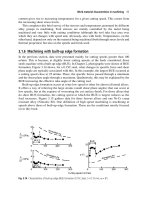
Fig. 1. MAPLSS−T
2
control chart.
206 Rosaria Lombardo, Amalia Vanacore and Jean-Francçois Durand
Fig. 2. Bar plot of contributions of process variables to the second dimension
Fig. 3. Bar plot of contributions of process variables to PMT .

regression procedure on each of them, having properly fixed the model parameters
(degree=1, knots=1, A=3). The computation of the T
2
scores for all Bootstrap sam-
ples allows to estimate the empirical distribution function of T
2
.Wefix the con-
trol chart upper and lower limits at the percentiles with D = 1% and D = 99%
(UCL=393.03, LCL=2.81)
Looking at the resulting control chart (see figure 1) we note two points out of control
at the beginning of the sequence (points 5 and 13). They must be investigated, using
bar plots (1) for points 5 and 13, the dimension 2 results as the most important one
for both out of control points. The bar plot (2) of process variables which contribute
MAPLSS-T
2
control chart 207
Table 1. MAPLSS results: R
2
according to the dimension
Dimension AR
2
%cum.
1 0.74 74%
2 0.16 89.6
3 0.03 92.3
to dimension 2 (figure 2) highlights that the most important process variables are the
temperature in zone 4 (T4 )zone3(T3), zone 2 (T2), zone 1 (T1), the interaction
between temperatures in zone 4 and zone 5 (T4*T5), ecc. In particular, T4 has a
strong effect on dimension 2 as well as on the quality product variable (Fig. 3). In
Fig. 3 we read in decreasing order the most important predictors on PMT, a part

from T4, the other important process variables are T1, T2, T6, T4*T5, and so on.
It is interesting to observe that the interaction between T4*T5 is more important
than the simple process variable given by T5 (Fig. 2 and 3). After the diagnosis
analysis, the causes for observed out of control points have been detected. In fact
the expert technologist suggests that the out-of-control signals are the consequence
of a ‘transition phenomenon’ due to a calibration problem in the feedback of the
automatic loop (i.e. the methane valve opens when temperature is naturally rising).
Having identified and removed the causes for the out of control signals, the modeling
phase of the MAPLSS-T
2
chart requires that the control limits should be recomputed
excluding the out of control points. The modeling phase ends when all points are
inside the control limits.
4 Conclusion
In this paper a powerful non-parametric multivariate process control chart has been
proposed for monitoring a manifacturing process. By simultaneously monitoring
process and product variables, MAPLSS-T
2
chart quickly detects and diagnoses un-
usual events that may occur during the process. The proposed non-parametric control
chart allows to handle collinear variables, missing values, outliers and interactions
between variables, without imposing any distributional assumption. Further devel-
opments of this work could be related to the construction of a chart of the Squared
Prediction Error (SPE; Kourti and MacGregor, 1996) on MAPLSS model, in order to
monitor any change in the covariance structure and verify that the process conditions
during the monitoring stage are not different with respect to the time the in control
MAPLSS model was developed.
References
CHAKRABORTI, S., VAN DER LAAN, P. and BAKIR, S.T. (2001): Nonparametric control
chart: an overview and some results. Journal of Quality Technology, 33, pp. 304-315.

208 Rosaria Lombardo, Amalia Vanacore and Jean-Francçois Durand
DURAND, J.F. (2001): Local Polynomial additive regression through PLS and splines: PLSS.
Chemiometric and Intelligent Laboratory systems, 58, pp. 235-246.
HAWKINS, D.M. (1991): Multivariate Quality Control based on regression-adjusted vari-
ables.Technometrics, 33, pp. 61-75.
HOTELLING, H. (1947): Multivariate Quality Control, in Techniques of Statistical Analysis.
Eds. Eisenhart, Hastay and Wallis, MacGraw Hill, New York.
JACKSON, J. E. (1991): A User Guide to Principal Component. Wiley, New York.
JONES, A. L. and WOODALL, W.H. (1998): The performance of Bootstrap Cotrol Charts.
Journal of Quality Technology, 30, pp. 362-375.
KOURTI, T. and MACGREGOR, J. F. (1996): Multivariate SPC Methods for Process and
Product Monitoring. Journal of Quality Technology, 28, pp. 409-428.
LIU, Y.R. (1995): Control Charts for Multivariate Processes. Journal of the American Statis-
tical Association, 90, pp. 1380-1387.
LIU, Y.R. and TANG, J. (1996): Control Charts for Dependent and Independent Measure-
ment based on Bootstrap Methods.Journal of the American Statistical Association, 91,
pp. 1694-1700.
LOMBARDO, R., DURAND, J.F., DE VEAUX, R. (2007): Multivariate Additive Partial
Least Squares via Splines. Submitted.
LOWRY, C. A., WOODALL, W. H., CHAMP, C. W., RIGDON, S. E. (1992): A multivariate
EWMA control chart. Technometrics, 34, pp. 46-53.
MACGREGOR, J.F. (1997): Using On-line Process Data to Improve Quality: Challenges for
Statisticians.International Statistical Review, 65, pp. 309-323.
NOMIKOS, P. and MACGREGOR, J.F. (1995): Multivariate SPC Charts for Monitoring
Batch Processes. Technometrics, 37, pp. 41-59.
TENENHAUS, M. (1998): La Règression PLS, Thèorie et Pratique. Eds. Technip, Paris.
VANACORE, A. and LOMBARDO, R. (2005): Multivariate Statistical Control Charts by non-
linear Partial Least Squares.Proceedings of Cladag 2005 conference, pp. 525-528.
WOLD, H. (1966): Estimation of principal components and related models by iterative least
squares. In Multivariate Analysis, (Eds.) P.R. Krishnaiah, New York: Academic Press, pp.

391-420.
WOODALL, W. H. and NCUBE, M. M. (1985): Multivariate CUSUM quality control proce-
dures. Technometrics, 27, pp. 285-292.
Nonlinear Constrained Principal Component Analysis
in the Quality Control Framework
Michele Gallo
1
and Luigi D’Ambra
2
1
Department of Social Science, University of Naples - L’Orientale
Largo S.Giovanni Maggiore 30, 80134 Naples, Italy

,
2
Department of Mathematics and Statistics, University of Naples - Federico II
Via Cinthia 26, 80126 Naples, Italy

Abstract. Many problems in industrial quality control involve n measurements on p process
variables X
n,p
. Generally, we need to know how the quality characteristics of a product behav-
ior as process variables change. Nevertheless, there may be two problems: the linear hypothe-
sis is not always respected and q quality variables Y
n,q
are not measured frequently because of
high costs. B-spline transformation remove nonlinear hypothesis while principal component
analysis with linear constraints (CPCA) onto subspace spanned by column X matrix. Linking
Y
n,q

and X
n,p
variables gives us information on the Y
n,q
without expensive measurements and
off-line analysis. Finally, there are few uncorrelated latent variables which contain the infor-
mation about the Y
n,q
and may be monitored by multivariate control charts. The purpose of
this paper is to show how the conjoint employment of different statistical methods, such as
B-splines, Constrained PCA and multivariate control charts allow a better control on prod-
uct or service quality by monitoring directly the process variables. The proposed approach is
illustrated by the discussion of a real problem in an industrial process.
1 Introduction
Frequently firms have to define how to select the process parameters which mostly
influence the quality characteristics of a product. The selection of the "optimal" com-
bination of parameters and the choice of statistical methods to solve this problem
could be no simple question. In this paper, we have proposed some statistical tech-
niques to determinate the "best" technology for pasta production.
Quality characteristics of pasta, tested in laboratory, can be divided in two clus-
ters: "colour-appeal" and "taste". Customers prefer clear and amber pasta without red
vein. Besides, the pasta must be characterise by "al dente" stage in case of overcook-
ing or undercooking (Abecassis et al., 1992).
In this paper, we suggest a nonlinear approach to select the "best" technology for
pasta production, spaghetti about 0.04 in (diameter), and choose process parameters
was to monitor.
194 Michele Gallo and Luigi D’Ambra
In the firststep,wedefine the different setting of the manufacturing process
which can be used. To obtain an optimal setting, it is necessary to consider three
process parameters: temperature (T) , drying time (DT), damp (D). Forty-five tests

have been running with different combinations of process parameters. At the same
time, quality characteristics have been measured by six variables: viscosity on a 1-9
category scale (V), judgement on taste in case of overcooking (N1) and undercooking
(N2) on a 0-9 category scale, homogeneity of red (A), yellow (B), brown (100-L). In
the second step, we define every new relation between response variables (Y
45,6
)and
process variables (X
45,7
) by-means of multivariate statistical methods such as Con-
strained Principal Component Analysis (CPCA - D’Ambra and Lauro, 1982). In the
third step, since CPCA analysis shows a horseshoes effect in data set, we propose a
B-spline transformation in data before interpreting results. In the last step, we define,
by means a Shewhart charts, the "optimal" combination of process parameters which
produces the "best" pasta.
The use of traditional control charts to monitor the process variables instead of
the response ones is a good solution for many reasons. First, the process variables
are measured much more frequently, usually in the order of seconds or minutes as
compared to hours for the response variables. Second, process variables are generally
measured in a more precise way than response variables. Third, CPCA components
are always independent even when single variables are correlated.
The aim of this paper is to show how the CPCA methods can be used in case of
nonlinear data and the employment of techniques like Multivariate Principal Com-
ponent Charts (MPCC - MacGregor and Kourti, (1995)) can aid in the interpretation
of results. The paper is organised as follows. In Section 2 CPCA method is applied to
pasta data. A horseshoes effect is present on raw data. Different approaches to solve
this problem is given in Section 3, in particular, B-spline transformation on X data is
applied. In Section 4 the results of CPCA on B-spline transformed data are tested by
a stability analysis. A first interpretation of CPCA results is given in Section 5.
2 Constrained principal component analysis

Let X
n,p
and Y
n,q
be the raw data matrices associated with two sets of quantitative
variables observed on the same experimental units. Furthermore let Q and D be sym-
metric and positive definite matrices of qth-order and nth-order respectively. In the
remainder of the paper, we will consider X and Y standardised data matrices, hence
Q = 1 . The CPCA (D’Ambra and Lauro, 1982) aim is to analyse the structure of the
explained variability of the Y data set given the process variables X.Let
P
X
= X(X

D
X
X)
−1
X

(1)
be the D-orthogonal projector onto the space spanned by the columns of X CPCA
consists in carrying out a PCA on the matrix

Y = P
X
Y (2)
Constrained Principal Component Analysis 195
Figure 1 shows a scatter plot of the first two principal components of the sta-
tistical study (


Y,D,I). It explain nearly all the data variability (87.80%) but in this
representation the second axis is a special arched function of the first axis. CPCA cre-
ates a serious artifact called the horseshoes effect. This is a problem because CPCA
perform better when the 45 experimental tests have a monotonic distributions along
gradients (i.e. either increase or decrease but not both). To resolves horseshoes prob-
lem and gives more interpretable results, nonlinear transformation of data can be
used (Gifi, 1990).
Fig. 1. Plot of the first and second Constrained Principal Component.
3 Nonlinear Constrained Principal Component Analysis
B-spline approach (Durand, 1993) allows a greater flexibility in the adjustment of
dependence between the X and Y sets of variables.
Let S
j
(x
j
)B
j
be the transformation of x
j
-column, j = 1, ,p , S
j
(n,k) the B-
basis spline with a priori fixed order and knots (De Boor, 1978; Eubank, 1988),
B
j
(k, q) is the matrix of coefficient.
Similarly we can write S as:
S
(n,


k)
=[S
1
(x
1
)| |S
p
(x
p
)] (3)
and B as:
B
(

k,q)
=
⎡
⎢
⎣
B
1
.
.
.
B
p
⎤
⎥
⎦

(4)
Consider the following multivariate model
196 Michele Gallo and Luigi D’Ambra
X = S

B +

E (5)
In order to estimate the

B we will minimise the trace

E


E.Then
min
B
X −S

B
2
(6)
Consider the class of reduced-rank regression for the multivariate linear model
with rank(

B)=r ≤ [min(6k,q)] (Izenman, 1975). With such condition there will
exist two (non-unique) matrices

B

r
=

A
r

G
r
where

A
r
and

G
r
are both of rank r.So
we have to minimise
min

A
r

G
r
X −S

A
r


G
r

2
(7)
The solutions for the minimisation of (7) are given by

G
r
=[v

1
v

r
],

A
r
=
(S

S)
−1
S

X[v
1
v
r

] where v
k
is the eigenvector corresponding to the k largest eigen-
value O
k
of Y

S(S

S)
−1
S

Y (Izenman, 1975).
The regression coefficient with rank r is therefore given by

B
r
=(S

S)
1
S

X[
r

k=1
v
k

v

k
] (8)
This solution is linked to an extension of CPCA, called CPCC-additive spline,
concerning a PCA of the image of y
j
onto B-basis spline with knots chosen in the
range of each y
j
, j = 1, ,p.Inthiscasewehave

Y
∗
= P
s
Y = S(S

S)
−1
S

Y and we
carrying out PCA of the statistical study (

Y
∗
,D, I).
A second approach (Durand, 1993) searches a matrix transformation C of X and
a matrix R to minimise the distance between the scalar product operators YY


D and
CRC

D:
min
C,R
YY

D −CRC

D
2
(9)
with C = S

B and where S is the B-spline matrix with a priori fixed order and
knots. The minimum can be attained by an approximate solution based on an alter-
nate iterative procedure.
A more recent method is the two-stage approach to engine mapping by using
B-spline basis functions at the second stage to describe the effects of one or more
factors (splined factors) and low-order monomials to represent the main effects and
interactions of the remaining (nonsplined) factors (Grove et al., 2004).
In this paper we have used the first approach. The first principal component of
the statistical study

Y
∗
,D, I explains the 81.10% of the total variation of the matrix Y.
The 96.80% of the total variance is explained by the first two principal components.

A stability analysis can be performed to evaluate the goodness of the results.
Constrained Principal Component Analysis 197
4 Stability analysis
Daudin (1988) suggests the study of stability by bootstrap. The basic idea of boot-
strap is to generate many new matrices starting from the raw data. Any new matrix
is obtained by a random replacement of the original rows. Applying bootstrap on

Y
∗
,
we generate m new matrices
l

Y
∗
where l = 1, ,m. Let O
i
and

z
i
be the ith eigen-
value and the associated eigenvector of the correlation matrix of

Y
∗
and
l

z

f
the fth
eigenvector of the correlation matrix of
l

Y
∗
. Furthermore let
l
U
if
= cos(
l

z
f
,

z
i
)=

O
i
l

z

f
,


z
i
(
l

z

f
,

z
f
)
1/2
(10)
and
l
J
k
= 6
i<k
6
f <k
l
U
2
if
(11)
where i, f = 1, ,k, and k is the number of the examined eigenvalues.

Plotting
l
J respect x-axis and j versus y-axis , the orientation of the first two
eigenvectors seems to be stable (Figure 2). In fact, it is not considerably modified
over the 250 replications.
Fig. 2. The stability representation for the first two eigenvectors.
The stability of the components can be confirmed by the following quantity
MSE(k)=
1
m
6
i<k
6
f <k
(
l
J
k
−k)
2
. (12)
If MSE(k) is near to zero, the examined k components are stable. Here for k = 2
and m = 250 the result is 0.000084.
5 Results and interpretation
Figure 3 shows the representation of 45 samples of the first two principal compo-
nents, where the percent of the total variability explained is 96.80. This percentage
198 Michele Gallo and Luigi D’Ambra
allows a good description of data structure and stability analysis indicates that this
data structure could be considered stable. Furthermore, the dotted lines show that B-
spline transformation have smoothed raw data and the problem of nonlinearity would

seem to be eliminated.
Fig. 3. Plot of the first and second Nonlinear Constrained Principal Component; the points are
the 45 different tests and the vectors are variables: temperature (T); drying time (DT); damp
(D); interaction between temperature, drying time and damp (T*DT*D); temperature and dry-
ing time(T*DT); temperature and damp (T*D); drying time and damp (DT*D); viscosity (V );
judgement on taste in case of overcooking (N1) and undercooking (N2); homogeneity of red
(A), yellow (B), brown (100-L).
The first axis of representation could be called "taste" as it is characterised by
contributions of viscosity and judgement on taste together with contributions of red
and brown colour. All these variables are positively correlated with "taste" (about
0.97). The second axis could be called "colour-appeal", as the yellow colour con-
tributes to this axis with 98%. The process variables which have a positive influence
on "taste" are temperature, drying time, their interaction and the interaction between
drying time and damp. On the contrary, all the other variables have a negative influ-
ence. The second axis is characterised mostly by the fact that drying time and damp
are each at the opposite side of the other, this contrast influences the homogeneity of
yellow.
The PCA of statistical study (

Y
∗
,D, I) indicates only which process variables
influence the quality characteristics of products. The direction where to look for the
best combination of process parameters (Abecassis et al., 1992) is along the diagonal
D-DT (Figure 3). This information could be not sufficient clear because along the
diagonal D-DT there are a lot of different combinations of process parameters. In
Constrained Principal Component Analysis 199
this case, a graphic display, such as Shewhart charts, could give some information
about the optimal combination to choose for the production of pasta.
The scores could be projected onto Shewhart charts where Central Line (CL),

Upper Decision Line (UDL) and Lower Decision Line (LDL) are 0, 0+3 and 0-3
respectively. In this paper, these "Multivariate Principal Component Charts" (MPCC)
are used for the first principal component (Figure 4.a), and the second one (Figure
4.b) or both, according to marketing decisions, that is maximise "taste" or "colour-
appeal" or choose the optimal mix of "taste" and "colour-appeal".
Fig. 4. MPCC for the first (a) and the second (b) Nonlinear Constrained Principal Component.
In Figure 4.a, the experimental tests 34, 38, 39, 40, 44 and 45 could suggest that
temperature must be higher than 100
◦
C to give the best value for "taste". Figure 4.b
shows that the best value for "colour-appeal" is obtained in correspondence of tem-
perature 90
◦
C, drying time 2.5 or 5, and damp 5.5. The "optimal" mixture of "taste"
and "colour-appeal" is obtained in correspondence of the maximum value taken in
Figure 4.b, by the experimental tests which are out of the UDL in Figure 4.a. The
experimental test 40 could be represents the "optimal" combination of parameters in
term of "taste" and "colour-appeal".
6 Concluding remarks
Today the advent of on-line process computer system have totally changed the nature
of the data that are available. The use of multivariate statistical methods is necessary
to treat the problems associated with these large volumes of messy data. We can use
all the information contained in data, to improve the quality of products and pro-
cesses. Multivariate analysis as Constrained Principal Component Analysis could be
employed to determine the relationships between the quality characteristic of prod-
ucts with the process parameters. In this way, we can select the best technology to get
a quality product and/or to monitor the quality characteristics of product by process
variables.
In many situation it is reasonable attend to the presence of anomalies observa-
tions, in these cases principal components are influenced and may not capture the

200 Michele Gallo and Luigi D’Ambra
variation of the regular observations. Therefore, data reduction based on PCA be-
comes unreliable. When outliers are present in the data, to obtain a more accurate
estimates at noncontaminated data sets and more robust estimates at contaminated
data a method for robust principal component analysis could be used (Hubert et al.,
2005).
References
ABECASSIS, J., DURAND, J.F., MEOT, J.M., and VASSEUR, P. (1992): Etude non linéaire
de l’influence des conditions de séchage sur la qualité des pâtes alimentaires par
l’analysis en composantes principales par rapport à des variables instrumentales. Agro-
Industrie et Methodes Statistiques, 3èmes Journees Europeennes.
D’AMBRA, L., and LAURO, N. (1982): Analisi in componenti principali in rapporto ad un
sottospazio di riferimento. Italian Journal of Applied Statistics,1.
DAUDIN, J.J., DUBY, C., and TRECOURT, P. (1988): Stability of stability of principal com-
ponent analysis studied by bootstrap method. Statistics , 19, 2.
DE BOOR, C. (1978): A practical guide to splines. Springer, N.Y.
DURAND, J.F. (1993): Generalized principal component analysis with respect to instrumental
variables via univariate spline trasformations. Computational Statistics Data Analysis,
16, 423-440.
EUBANK, R.L. (1988): Smoothing splines and non parametric regression. Markel Dekker
and Bosel, N.Y.
GIFI, A. (1990): Nonlinear Multivariate Analysis. Wiley, Chichester, England.
GROVE, D.M., WOODS, D.C., and LEWIS, S.M. (2004): Multifactor B-Spline Mixed Mod-
els in Designed Experiments for the Engine Mapping Problem. Journal of Quality Tech-
nology, 36, 4, 380-391.
IZERNMAN, A.J. (1975): Reduced-rank regression for the multivariate linear model. Journal
of Multivariate Analysis,5.
HUBERT, M., ROUSSEEUW, P.J., and BRANDEN, K.V. (2005): ROBPCA: A New Ap-
proach to Robust Principal Component Analysis. Technometrics, 47, 1.
MACGREGOR, J.F. and KOURTI, T. (1995): Statistical Process Control of Multivariate Pro-

cesses. Control Engineering Practice, 3, 3, 403-414.
Simple Non Symmetrical Correspondence Analysis
Antonello D’Ambra
1
, Pietro Amenta
1
and Valentin Rousson
2
1
University of Sannio, Benevento, Italy
{andambra, amenta}@unisannio.it
2
Department of Biostatistics, University of Zürich, Switzerland

Abstract. Simple Component Analysis (SCA) was introduced by Rousson and Gasser (2004)
as an alternative to Principal Component Analysis (PCA). The goal of SCA is to find the
“optimal simple system” of components for a given data set, which may be slightly correlated
and suboptimal compared to PCA but which is easier to interpret.
Aim of the present paper paper is to consider an extension of SCA to categorical data.
In particular, we consider a simple version of the Non Symmetrical Correspondence Analy-
sis (D’Ambra and Lauro, 1989). This latter approach can be seen as a centered PCA on the
column profile matrix with suitable metrics enabling to describe the association in two way
contingency table in cases where one categorical variable is supposed to be the explanatory
variable and the other the response.
1 Introduction
It is well known that Principal Component Analysis (PCA) is optimal in at least
two ways: principal components extract a maximum of the variability of the original
variables and they are uncorrelated. The former ensures that a minimum of “total
information” will be missed when looking at the first few principal components. The
latter warrants that the extracted information will be organized in an optimal way:

we may look at one principal component after the other, separately, without taking
into account the rest.
Unfortunately, principal components often lack interpretability. They define some
abstract scores which often are not meaningful, or not well interpretable in practice.
The same remark applies to all methods based on PCA.
Simple Component Analysis (SCA) was introduced by Rousson and Gasser
(2004) as an alternative to Principal Component Analysis. The goal of SCA was to
find the “optimal simple system” of components for a given data set. A component
was considered to be simple if the number of possibles values for its loadings was
restricted to three (a positive one, zero and a negative one). Optimality of a syztem of
components was defined as in Gervini and Rousson (2004). At the end, the optimal
210 Antonello D’Ambra, Pietro Amenta and Valentin Rousson
simple system defined by SCA may be slightly correlated and suboptimal compared
to PCA but will be easier to interpret. Thus, SCA may represent a worth alternative
to PCA if the loss of optimality remains modest.
Aim of the present paper is to consider an extension of SCA to categorical data.
In particular, we consider a simple version of the Non Symmetrical Correspondence
Analysis (D’Ambra and Lauro, 1989). This latter approach can be seen as a PCA
performed on the column profile matrix with the same weighting system of Corre-
spondence Analysis but in a different metric.
Advantages of the method are illustrated with a well known data set.
2 Non symmetrical correspondence analysis
In many fields, the researcher is interested to study the relationship between two or
more variables. When the variables are collected in a contingency table, classical
statistic tools like correspondence analysis (CA) are applied in order to measure and
visualize the strength of the association.
The CA is based on the decomposition of the index I
2
of Pearson, which is a
symmetric measure of association. This approach however is no longer appropriate

when one has to study a two way contingency table where one categorical variable is
supposed to be the explanatory variable and the other the response. To overcome this
problem, D’Ambra and Lauro (1989) introduced the Non Symmetrical Correspon-
dence Analysis (NSCA). This approach decomposes the numerator of the Goodman-
Kruskal W (1954), which is an asymmetric measure of association in a contingency
table.
Given two categorical variables I and J, the goal of NSCA is to evaluate the
influence of categories of the explanatory variable J on the distribution of the reponse
I.
Let N =(n
ij
) and P =
N
n
=(p
ij
)=(
n
ij
n
) be the absolute and relative two-way con-
tingency table of dimension I ×J where I and J also denote the number of categories
of the response and the explanatory variable, respectively, based on n individuals. Let
p
i.
=

J
j=1
p

ij
and p
. j
=

I
i=1
p
ij
be the column and row marginals, respectively,
and let D
j
= diag(p
. j
).
Finally, let
3 =(S
ij
)=(
p
ij
p
. j
−p
i.
)
be the matrix describing the conditional distribution of I given J. This matrix contains
information on the I conditional distributions
p
ij

p
. j
adjusted to the row marginal p
i.
,and
is hence a weighted average of the column profiles.
From a geometrical point of view, the purpose of NSCA is to evaluate in the space
R
I
the spread of the cloud of points defined by 3 around its centroid according to an
appropriate weighting system. A global measure of dispersion is given by the inertia
In = W
num
=
I

i=1
J

j=1
p
. j

p
ij
p
. j
−p
i.


2
.
Simple Non Symmetrical Correspondence Analysis 211
NSCA looks for the orthonormal basis which accounts for the largest part of iner-
tia to visualize the dependence structure between J and I in a lower dimensional
space. Solutions are given by the eigen-analysis of the variance covariance matrix
S = 3D
j
3

whose general term (i,i

) is given by
s
ii

=
J

j=1
p
. j

p
ij
p
. j
−p
i.


p
i

j
p
. j
−p
i

.

where p
i.
denotes the centre of gravity of the ith row of P. This is achieved also by
the generalized singular value decomposition of 3 =

M∗
m=1
O
m
a
m
b
m

with M∗≤
M = min[(I, J) −1] and where the scalar O
m
is the singular value (we shall note
' = diag(O

m
)), a
m
and b
m
are orthonormal singular vectors in an unweighted and
weighted metric, respectively, such that a

m
a
m
= 1, a

m
a
m

= 0andb

m
D
j
b
m
= 1,
b

m
D
j

b
m

= 0 for m ≡ m

.
In the previous decomposition, the numerator of the Goodman and Kruskal W
(1954) can be decomposed as W
num
=

M∗
m=1
O
2
m
.
The factorial row and column coordinates are given by \
m
=
√
O
m
a
m
and M
m
=
√
O

m
D
−1/2
j
b
m
, respectively. Finally, factorial coordinates can be also obtained from
the transition formulae:
M
m
=

1
√
O
m


i

p
ij
p
. j
−p
i.

\
m
\

m
=

1
√
O
m


j
p
. j

p
ij
p
. j
−p
i.

M
m
See D’Ambra and Lauro (1989) for further details and remarks.
3 Simple non symmetrical correspondence analysis
It is possible to show that NSCA corresponds to a PCA of the profile matrix 3 with
suitable row and column metrics. This is equivalent (Tenenhaus and Young, 1985) to
study the statistical triplet (3, I,D
j
) where the identity matrix I denotes the metric
and D

j
the weighting system. Thus, like all PCA-based methods, the components
produced by NSCA are optimal but may lack interpretability, as recalled in the In-
troduction.
In the similar way as SCA was introduced as an alternative to PCA, we shall now
introduce a technique called Simple NSCA as an alternative to NSCA. For this, we
shall use similar concepts and algorithms as in SCA. Note that while one makes the
distinction between simple block-components and simple difference-components in
SCA, we shall here consider only difference components (i.e. components with both
positive and negative loadings), since NSCA does not produce block-components
(i.e. components where all loadings share the same sign). Thus, we shall consider
simple components with loadings proportional to vectors with only three different