Data Analysis Machine Learning and Applications Episode 1 Part 10 ppt

212 Antonello D’Ambra, Pietro Amenta and Valentin Rousson
values (a negative value, zero, and a positive value), the sum of the loadings being
zero for each component (defining hence proper contrasts of categories).
The goal of Simple NSCA is to find the optimal system of components among
the simple ones, where optimality is calculated according to Gervini and Rousson
(2004).
The percentage of extracted variability V(L) accounted by a system L of m =
min(I,J) −1 components is given by
V(L)=
l

1
Sl
1
tr(')
+
1
tr(')
m

k=2
l

k

S −SL
(k−1)
(L

(k−1)
SL

(k−1)
)
−1
L

(k−1)
S

l
k
,
where l
k
is the kth column of L, and where L
(k−1)
is the m×(k−1) matrix containing
the first (k −1) columns of L.
Whereas the numerator of the first term of this sum is equal to the variance of the
first component, the numerator of the kth term can be interpreted as the variance of
the part of the kth component which is not explained by (which is independent from)
the previous (k−1) components. Thus, correlations are "penalized" by this criterion
which is hence uniquely maximized by PCA, i.e. by taking L = E
m
, the matrix of the
first m eigenvectors of S (Gervini and Rousson, 2004). The optimality of a system L
is then calculated as V(L)/V(E
m
).
In our sequential algorithms below, the k th simple component is obtained by
regressing the original row/column categories on the previous k −1 simple compo-

nents already in the system, by computing the first eigenvector of the residual vari-
ance hence obtained, and by shrinking this eigenvector towards the simple difference
component which maximizes optimality. Here are two algorithms providing simple
components for the rows and the columns.
Simple solutions for the rows
1. Let S = 3D
j
3

,letL be an empty matrix and let
ˆ
S = S.
2. Let a =(a
1
, ,a
I
)

be the first eigenvector of
ˆ
S.
3. For each cut-off value among g = {0, |a
1
|, ,|a
I
|}, consider the shrunken vector
b(g)={b
1
(g), ,b
I

(g)}

with elements b
k
(g)=sign(a
k
) if |a
k
|> g and b
k
(g)=
0 otherwise (for k = 1, ,I). Update and normalize it such that

b
k
(g)=0 and

b
2
k
(g)=1.
4. Include into the system the difference component b(g) which maximizes
b(g)

ˆ
Sb(g) (i.e. add the column b(g) to the matrix of loadings L).
5. If the maximum number of components is attained stop. Otherwise let
ˆ
S = S −
SL(L


SL)
−1
L

S and go back to step 2.
Simple solutions for the columns
1. Let S = D
1/2
j
3

3D
1/2
j
,letL be an empty matrix and let
ˆ
S = S.
2. Let a =(a
1
, ,a
J
)

be the first eigenvector of
ˆ
S.
Simple Non Symmetrical Correspondence Analysis 213
3. For each cut-off value among g = {0,|a
1

|, ,|a
J
|}, consider the shrunken vector
b(g)={b
1
(g), ,b
I
(g)}

with elements b
k
(g)=sign(a
k
) if |a
k
|> g and b
k
(g)=
0 otherwise (for k = 1, ,J). Update and normalize it such that

b
k
(g)=0and

b
2
k
(g)=1.
4. Include into the system the difference component b(g) which maximizes
b(g)


ˆ
Sb(g) (i.e. add the column b(g) to the matrix of loadings L).
5. If the maximum number of components is attained, let L = D
−1/2
j
L and stop.
Otherwise let
ˆ
S = S −SL(L

SL)
−1
L

S and go back to step 2.
4 Father’s and son’s occupations data
To illustrate the technique of Simple NSCA, we applied it to the well known Father’s
and Son’s Occupations. This data set (Perrin, 1904) was collected to study whether
and how the professional occupation of some man depends on the occupation of his
father. Occupations of 1550 men were cross-classified according to father’s and son’s
occupation reparted into 14 occupations.
The conclusion of the study was that such a dependence existed. Two measures
of predicability, the Goodman-Kruskal’s W (1954) and the Light and Margolin’s C =
(n −1)(I −1)W (1971), have been computed. Note that the C-statistic can be used
to formally test for association, being asymptotically chi-squared distributed with
(I −1)(J −1) degrees of freedom under the hypothesis of no association (Light and
Margolin, 1971).
The overall increase in predicability of a man’s occupation when knowing the oc-
cupation of his father was equal to 14% (W = 0.14; C = 2880.8; df = 169,

p
value
0.0001).
According to the NSCA decomposition of the numerator of W (W
num
=

M
k=1
O
2
k
=
0.1288), we have for the first two axes O
1
= 0.24 and O
2
= 0.16, which are the
weights of the axes in the joint plot of Figure 1. The first axis accounts for 100 ×
(0.24)
2
/0.1288 = 43.7% of the dependence between the two variables while the
second one represents 20.7%. Therefore Figure 1 accounts for 64.4% of the total
inertia.
Unfortunately, the two-dimensional NSCA solution (Figure 1) does not give a
clear description of the dependence of the two variables as well as of the association
between rows and columns. Thus, NSCA is difficult to interpret and a simple solution
has been calculated according to Simple NSCA.
From Table 1, one can see that the first component defined by Simple NSCA for
the rows contrasts son’s occupation “Art” versus the group of occupations {Army,

Divinity, Law, Medicine, Politics & Court and Scholarship & Science}. This simple
component explains 42.5% of the variance compared to 43.7% for optimal solution
above. Thus, the first simple row solution is 42.5%/43.7%=97.4% optimal. One can
conclude that the influence of father’s occupation on son’s occupation mainly con-
trasts these two groups of occupation. The second simple row solution provided by
Simple NSCA contrasts son’s occupation “Divinity” versus the group of occupations
{Army and Politics & Court}.
214 Antonello D’Ambra, Pietro Amenta and Valentin Rousson
Fig. 1. Non Symmetrical Correspondence Analysis (NSCA): Joint plot.
The same table also contains the Simple NSCA solution for the columns. The
first simple column solution contrasts father’s occupation “Art” versus “Divinity”,
and is 81.9% optimal. The second simple column solution contrast groups of father’s
occupations {Army, Landownership, Law and Politics & Court} versus {Art and
Divinity} with an optimality value of 90.4%. Similarly, further simple constrats can
be defined for both the rows and the columns (see Table 1 for the first 5 solutions).
Simple Non Symmetrical Correspondence Analysis 215
Table 1. Simple NSCA solutions for the first five axes.
SON (row) FATHER (column)
Axis1 Axis2 Axis3 Axis4 Axis5 Axis1 Axis2 Axis3 Axis4 Axis5
Army 0,15 -0,41 -0,44 -0,37 -0,50 0,00 -0,89 -1,20 3,21 0,00
Art -0,93 0,00 0,00 0,00 0,00 -2,04 1,77 -1,20 0,00 0,00
TCCS 0,00 0,00 0,00 0,00 0,00 0,00 0,00 0,00 0,00 0,00
Crafts 0,00 0,00 0,00 0,00 0,00 0,00 0,00 0,86 0,00 0,00
Divinity 0,15 0,82 -0,44 0,00 0,00 2,04 1,77 -1,20 0,00 0,00
Agricolture 0,00 0,00 0,00 0,00 0,00 0,00 0,00 0,86 0,00 0,00
Landownership 0,00 0,00 0,00 0,00 0,00 0,00 -0,89 -1,20 0,00 0,00
Law 0,15 0,00 0,33 0,55 -0,50 0,00 -0,89 0,86 -1,61 -2,65
Literature 0,00 0,00 0,33 0,00 0,00 0,00 0,00 0,86 0,00 0,00
Commerce 0,00 0,00 0,33 0,00 0,00 0,00 0,00 0,86 0,00 0,00
Medicine 0,15 0,00 0,00 -0,37 0,50 0,00 0,00 0,86 0,00 2,65

Navy 0,00 0,00 0,00 0,00 0,00 0,00 0,00 0,00 0,00 0,00
POLCOURT 0,15 -0,41 -0,44 0,55 0,50 0,00 -0,89 -1,20 -1,61 0,00
SCSCIENCE 0,15 0,00 0,33 -0,37 0,00 0,00 0,00 0,86 0,00 0,00
Explained variance (%)
Optimal solu-
tion
43,70 64,40 75,30 83,00 89,20 43,70 64,40 75,30 83,00 89,20
Simple solu-
tion
42,50 62,20 72,30 79,70 85,70 35,80 58,20 68,50 75,10 80,30
Optimality 97,40 96,60 96,10 96,10 96,10 81,90 90,40 91,00 90,50 90,00
Note: TCCS, POLCOURT and SCSCIENCE stand for “Teacher, Clerck and Civil
Servant”, “Politics & Court” and “Scolarship & Science”, respectively.
To better summarize and visualize the relationship between father’s and son’s
occupation, it is helpful to plot the solutions for rows and columns for each axis on a
same graphic (Figure 2). One can see that the first Simple NSCA solution highlights
the fact that a son has the tendency to choose the same occupation as his father if
this occupation is “Art”, while father’s occupation “Divinity” is linked with a son’s
occupation within {Army, Divinity, Law, Medicine, Politics & Court and Scholarship
& Science}. Similarly, one can try to interpret the second Simple NSCA solution.
In summary, Simple NSCA provides a clearcut picture of the situation, the opti-
mality of the first two axes being in this example of more than 95% (for the rows)
and 90% (for the columns). Thus, the price to pay for simplicity is about 5% (for the
rows) and 10% (for the columns), which is not much. In this sense, Simple NSCA
may be a worth alternative to NSCA.
5 Conclusions
In general, all PCA-based methods are tuned to condense information in an optimal
way. However, they define some abstract scores which often are not meaningful or
not well interpretable in practice. This was also the case in our example above for
216 Antonello D’Ambra, Pietro Amenta and Valentin Rousson

Fig. 2. Summary of Simple NSCA solutions for the axes 1 and 2.
NSCA. To enhance interpretability, Simple NSCA focus on simplicity and seeks
for “optimal simple components”, as illustrated in our example. It provides a clear-
cut interpretation of the association between rows and columns, the price to pay
for simplicity being relatively low. In this sense, Simple NSCA may be a worth
alternative to NSCA. Extensions of this approach for the Classical Correspondence
Analysis and for ordinal variables are under investigation.
Simple Non Symmetrical Correspondence Analysis 217
References
D ’AMBRA, L. and LAURO, N.C. (1989): Non symmetrical analysis of three-way contin-
gency tables. In: R. Coppi and S. Bolasco (Eds.): Multiway Data Analysis. North Hol-
land, 301–314.
LIGHT, R. J. and MARGOLIN, B. H. (1971): An analysis of variance for categorical data.
Journal of the American Statistical Association, 66, 534–544.
GERVINI, D. and ROUSSON, V. (2004): Criteria for evaluating dimension-reducing compo-
nents for multivariate data. The American Statistician, 58, 72–76.
GOODMAN, L. A. and KRUSKAL, W. H. (1954): Measures of association for cross-
classifications. Journal of the American Statistical Association, 49, 732–7644.
PERRIN, E. (1904): On the Contingency Between Occupation in the Case of Fathers and
Sons. Biometrika, 3, 4, 467–469.
ROUSSON, V. and GASSER, Th. (2004): Simple component analysis. Applied Statistics, 53,
539–555.
TENENHAUS, M. and YOUNG, F.W., (1985): An analysis and synthesis of multiple cor-
respondence analysis, optimal scaling, dual scaling and other methods for quantifying
categorical multivariate data. Psychometrika, 50, 90–104.
A Comparative Study on Polyphonic Musical Time
Series Using MCMC Methods
Katrin Sommer and Claus Weihs
Lehrstuhl für Computergestützte Statistik,
Universität Dortmund, 44221 Dortmund, Germany

Abstract. A general harmonic model for pitch tracking of polyphonic musical time series will
be introduced. Based on a model of Davy and Godsill (2002) the fundamental frequencies
of polyphonic sound are estimated simultaneously. For an improvement of these results a
preprocessing step was be implemented to build an extended polyphonic model.
All methods are applied on real audio data from the McGill University Master Samples
(Opolko and Wapnick (1987)).
1 Introduction
The automatic transcription of musical time series data is a wide research domain.
There are many methods for the pitch tracking of monophonic sound (e.g. Weihs and
Ligges (2006)). More difficult is the distinction of polyphonic sound because of the
properties of the time series of musical sound.
In this research paper we describe a general harmonic model for polyphonic mu-
sical time series data, based on a model of Davy and Godsill (2002). After trans-
forming this model to an hierarchical bayes model the fundamental frequencies of
this data can be estimated with MCMC methods.
Then we consider a preprocessing step to improve the results. For this, we intro-
duce the design of an alphabet of artificial tones.
After that we apply the polyphonic model to real audio data from the McGill Uni-
versity Master Samples (Opolko and Wapnick (1987)). We demonstrate the building
of an alphabet on real audio data and present the results of utilising such an alphabet.
Further, we show first results of combining the preprocessing step and the MCMC
methods. Finally the results are discussed and an outlook to future work is given.
2 Polyphonic model
In this section the harmonic polyphonic model will be introduced and its components
will be illustrated. The model is based on the model of Davy and Godsill (2002) and
has the following structure:
286 Katrin Sommer and Claus Weihs
0.000 0.005 0.010 0.015 0.020
time (in sec.)

Ŧ10 1
amplitude
Fig. 1. Illustration of the modelling with basis functions. Modelling time-variant amplitudes
of a real audio signal
y
t
=
K

k=1
H

h=1
I

i=0
I
t,i

a
k,h,i
cos(2Shf
k
/ f
s
t)+b
k,h,i
sin(2Shf
k
/ f

s
t)

+ H
t
,
The number of observations of the audio signal y
t
is T, t ∈{0, ,T −1}. Each signal
is normalized to [−1,1] since the absolute overall loudness of different recordings is
not relevant. The signal y
t
is made up of K tones each composed out of harmonics
from H
k
partial tones. In this paper the number of tones K is assumed to be known.
The first partial of the k-th tone is the fundamental frequency f
k
, the other H
k
−1
partials are called overtones. Further, f
s
is the sampling rate.
To reduce the number of parameters to be estimated, the amplitudes a
k,h,t
and
b
k,h,t
of the k−th tone and the h-th partial tone at each timepoint t are modelled with

I + 1 basis functions. The basis functions I
t,i
are equally spaced hanning windows
with 50% overlap:
I
t,i
:= cos
2
[S(t −i')/(2')]1
[(i−1)',(i+1)']
(t), ' =(T −1)/I.
So the a
k,h,i
and b
k,h,i
are the amplitudes of the k-th tone, the h-th partial tone and the
i-th basis function. Finally, H
t
is the model error.
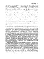
Figure 1 shows the necessity of using basis functions and thus modelling time-
variant amplitudes. In the figure the points are the observations of the real signal. The
assumption of constant amplitudes over time cannot depict the higher amplitudes at
the beginning of the tone (black line). Modelling with time-variant amplitudes (grey
line) leads to better results.
The model can be written as a hierarchical bayes model. The estimation of the pa-
rameters results from stochastic search for the best coefficients in a given region with
different prior distributions. The region and the probabilities are specified by distri-
butions. This leads to the implementation of MCMC methods (Gilks et al. (1996)).
Polyphonic Musical Time Series 287
For the sampling of the fundamental frequency f

k
variants of the Metropolis-
Hastings-Algorithm are used where the candidate frequencies are generated in dif-
ferent ways.
In the first variant the candidate for the fundamental frequency is sampled from
a uniform distribution in the range of the possible frequencies. In the second variant
the new candidate for the fundamental frequency is the half or the double frequency
of the actual fundamental frequency. In the third variant a random walk is used which
allows small changes of the fundamental frequency f
k
to get a more precise result.
For the determination of the number of partial tones H
k
a reversible jump MCMC
was implemented. In each iteration of the MCMC-computation one of these algo-
rithms is chosen with a distinct probability.
The parameters of the amplitude a
k,h,i
and b
k,h,i
are computed conditional on the
fundamental frequency f
k
and the number of partial tones H
k
.
There is no full generation of the posterior distributions due to the computational
burden. Instead we use a stopping criterion to stop the iterations if the slope of the
model error is no longer significant (Sommer and Weihs (2006)).
3 Extended polyphonic model

An extented polyphonic model with an additional preprocessing step to the MCMC-
algorithms will be established in this section. The results of this step could be the
starting values for the MCMC algorithm in order to improve the results.
For this purpose we constructed an alphabet of artificial tones. These artificial
tones are compared with the audio data to be analysed. The artificial tones are com-
posed by evaluating the periodograms of seven time intervals with 512 observations
of a real audio signal with 50% overlap. So a time interval of 2048 observations is re-
garded. At a sampling rate of 11 025 Hz a time interval of 0.186 seconds is observed.
These seven periodograms are averaged to a mean periodogram. For better com-
parability all values in this periodogram are set to zero which are smaller than one
percent of the maximum peak. All artificial tones together form the alphabet.
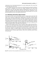
In figure 2 (upper part) a periodogram of a c4 (262 Hz) played by an electric
guitar can be seen. The lower part of figure 2 shows the small values of the peri-
odogram. The horizontal line reflects the value of one percent of the maximum value
of the periodogram. All values below this line are set to zero in the alphabet.
To determine the correct notes, every combination of two artificial tones of the
alphabet is matched to the periodogram of the real audio signal. The modified pe-
riodograms of the two artificial tones are summed up to one periodograms. These
periodograms are compared with the audio signal. The notes corresponding to the
two artificial tones which cause minimal error are considered as estimates for the
true notes. Finally, voting over ten time intervals leads to the estimation of the fun-
damental frequencies.
288 Katrin Sommer and Claus Weihs
0 500 1000 1500 200
0
0.00 0.10 0.20 0.30
Frequency
normalized periodogram
0 500 1000 1500 200
0

0.000 0.004 0.008
Frequency
normalized periodogram
Fig. 2. Periodogram of note c4 played with an electric guitar. Original (upper part) and zoomed
in with cut-off line (lower part)
4 Results
In this section results of estimating the fundamental frequencies of real audio data
will be figured out. First, the data used in our studies will be introduced. Then first
results are shown. Further the construction of an alphabet will be reconsidered and
then the results based on this alphabet are depicted. Finally additional results are
shown.
4.1 Data
The data used for our monophonic and polyphonic studies are real audio data from
the McGill University Master Samples (Opolko and Wapnick (1987)). We chose 5
instruments (electric guitar, piano, violin, flute and trumpet) each with 5 notes (262,
Polyphonic Musical Time Series 289
Table 1. 1 if both notes were correctly identified, 0 otherwise. The left hand table requires the
exact note to be estimated, the right table also counts octaves of the note as correct.
instrument
notes flu guit pian trum viol
c4–c4 1 1 1 1 1
c4–e4 0 1 0 0 1
c4–g4 0 0 0 0 0
c4–a4 1 1 1 0 0
c4–c5 1 1 1 1 1
instrument
notes flu guit pian trum viol
c4–c4 1 1 1 1 1
c4–e4 0 1 0 1 1
c4–g4 1 1 1 1 1

c4–a4 1 1 1 0 0
c4–c5 1 1 1 1 1
330, 390, 440 and 523 Hz) out of two groups of instruments, string instruments and
wind instruments. The three string instruments are played in different ways, namely
picked, struck and bowed. The two wind instruments are a woodwind instrument and
a brass instrument.
For polyphonic data we superimposed the oszillations of two tones. The first
tone was a c4 (262 Hz) played by the piano. This tone was combined with each
instrument–tone combination we used. So we had 25 datasets each normalized to
[−1,1]. The pitches of the tones were tracked over ten time intervals of T = 512
observations with 50% overlap at a sampling rate of 11 025 Hz. The number of ob-
servations in one time interval is a tradeoff between the computational burden and
the quality of the estimate. The estimate of the notes is the result of voting over the
ten time intervals. The estimated notes are the two notes which occur in the ten time
intervals most often.
4.2 First results with polyphonic model
The first step in our analysis was to consider how good the model works and if the
pitch of a tone is estimated exactly. For this purpose we made a first study with
monophonic data. The results of the study with monophonic time series data were
very promising. In most cases the correct note was estimated and the deviations from
the correct fundamental frequencies were minor (Sommer and Weihs (2006)).
The results of the estimation of polyphonic time series data are not as promising
as the results with monophonic time series data. There are many notes which are not
estimated correctly. The left side of Table 1 shows 1 if both notes were estimated
correctly and 0 otherwise. In 15 of the 25 experiments both notes were estimated
correctly. Counting octaves of the notes as correct increases the number of correct
estimates to 21 (see the right hand side of Table 1). It can be seen that all notes of
the combination c4–g4 are estimated incorrectly, but they are correct by counting the
octaves of the right notes as correct (Sommer and Weihs (2007)).
Analysing the data over 20, 30 and 50 time intervals results in the same outcomes.

So it seems to be adequate to examine 10 time intervals. In longer interval series new
correctly estimated notes could not be determined.
290 Katrin Sommer and Claus Weihs
Table 2. 1 if both notes AND instruments are correctly recognized after voting and 1
∗
if both
notes are estimated correcty, but not the instrument (left), including octaves of the correct
notes (right). In 22 (left) and 23 (right) cases both notes are estimated correctly, in 18 cases
for both tones the correct instrument is recognized.
instrument
notes flu guit pian trum viol
c4–c4 0 0 1
∗
1
∗
1
c4–e4 1 1 1 1 1
∗
c4–g4 1 1 1 1 1
c4–a4 1 1 1 1 1
c4–c5 1 1 0 1
∗
1
instrument
notes flu guit pian trum viol
c4–c4 0 0 1
∗
1
∗
1

c4–e4 1 1 1 1 1
∗
c4–g4 1 1 1 1 1
c4–a4 1 1 1 1 1
c4–c5 1 1 1
∗
1
∗
1
4.3 Results with extended polyphonic model
In a first study with an alphabet of artificial tones we used 30 notes from g3 (196 Hz)
to c6 (1 047 Hz) of the same five instruments as for the studies in section 4.2. The
choice of this range is restricted by the availability of the data of the McGill Univer-
sity Master Samples. The mean periodogram is computed out of seven periodograms
each with T = 512 observations with 50% overlap at a sampling rate of 11 025 Hz.
The first 1000 observations of a note were not considered for this periodogram in
order to omit the attack of an instrument. Overall there are 150 artificial notes in the
alphabet.
With this alphabet 11 325 pairwise comparisons of two artificial tones with the
audio signal have to be computed. The results of the estimates of the same 25 note-
combinations used in the previous study can be seen in table 2. The left hand side
of the table shows that in 22 of 25 cases the fundamental frequency of both notes is
estimated correctly. If octaves of the correct notes are counted as correct this number
increases to 23 (right hand side of table 2).
Further, the entries in table 2 are annotated with a star if the instruments are not
recognized correctly. This means that only in 18 of 22 cases (18 of 23) the instru-
ments of both notes are identified correctly. Moreover, it can be seen that the cases
where the notes are estimated incorrectly occur only in the first and last rows of the
tables. So the correct estimation of the notes seems to be a problem if both notes are
the same or one is the octave of the other.

4.4 Further results
Using these estimated notes as starting values for the MCMC algorithm in order to
estimate the fundamental frequencies more precisely does not lead to an improve-
ment of the results of the preprossing. To the contrary, the results are comparable to
the results without this preprocessing step. In most of the cases the estimated notes
are the octave of the correct notes. Often, the MCMC algorithm leads to an esti-
mate
ˆ
H = 1 of the number of partial tones. This often meant that only the octave of
Polyphonic Musical Time Series 291
the fundamental frequency is found and neither the fundamental itself nor any other
overtones.
A solution to this problem is the limitation of the possible range of frequencies.
Restricting the frequency to the same range which the alphabet is covering and forc-
ing the number of partial tones to be greater than 1 yields 20 respectively 24 correct
estimations of both notes. A further improvement can be achieved by applying two
chains in the MCMC algorithm. Starting values for both chains are equal, namely
the results of the preprocessing. For each time interval the chain with the minimal
model error is chosen. Voting over the ten time intervals results in 22 respectively 25
correct estimates. There are no more incorrectly estimated notes, in the worst case
octaves of the correct notes. Also, voting is based on many more correct notes in the
individual time intervals of 512 observations than in our previous studies, i.e. now
typically five or six estimates are correct in contrast to three before.
5 Conclusion
In this paper a pitch tracking model for polyphonic musical time series data has
been introduced. The unknown parameters are estimated with an MCMC algorithm
as a stochastic optimization procedure. Because of the unfavorable results in a first
study with polyphonic data the polyphonic model was extended and a preprocessing
step was implemented. The application of an alphabet of artificial notes leads to
promising results. The combination of the preprocessing and the MCMC algorithm

is even more encouraging after the limitation of the frequency range.
Further work will extend the alphabet by using more artificial tones and consid-
ering attack, sustain and release, the different phases of a realisation of a note. An
additional aim is the construction of a complete alphabet on the whole audio data of
the McGill Universitiy Master Samples.
Acknowledgements
This work has been supported by the Graduiertenkolleg “Statistical Modelling” of
the German Research Foundation (DFG).
References
DAVY, M. and GODSILL, S. J. (2002): Bayesian Harmonic Models for Musical Pitch Estima-
tion and Analysis. Technical Report 431, Cambridge University Engineering Department.
GILKS, W. R., RICHARDSON, S. and SPIEGELHALTER D. J. (1996): Markov Chain Monte
Carlo in Practice, Chapman & Hall.
OPOLKO, F. and WAPNICK, J. (1987): McGill University Master Samples [Compact disc]:
Montreal, Quebec: McGill University.
SOMMER K. and WEIHS C. (2006): Using MCMC as a stochastic optimization procedure
for music time series. In: V. Batagelj, H.H. Bock, A. Ferligoj, and A. Ziberna (Eds.):
Data Science and Classifiction , Springer, Heidelberg, 307–314.
292 Katrin Sommer and Claus Weihs
SOMMER K. and WEIHS C. (2007): Using MCMC as a stochastic optimization procedure
for monophonic and polyphonic sound. In: R. Decker and H. Lenz (Eds.): Advances in
Data Analysis, Springer, Heidelberg, 645–652.
WEIHS, C. and LIGGES, U. (2006): Parameter Optimization in Automatic Transcription of
Music. In: Spiliopoulou, M., Kruse, R., Nürnberger, A., Borgelt, C. and Gaul, W. (eds.):
From Data and Information Analysis to Knowledge Engineering. Springer, Berlin, 740 –
747.
A Matlab Toolbox for
Music Information Retrieval
Olivier Lartillot, Petri Toiviainen and Tuomas Eerola
University of Jyväskylä, PL 35(M), FI-40014, Finland

Abstract. We present MIRToolbox, an integrated set of functions written in Matlab, dedicated
to the extraction from audio files of musical features related, among others, to timbre, tonality,
rhythm or form. The objective is to offer a state of the art of computational approaches in the
area of Music Information Retrieval (MIR). The design is based on a modular framework: the
different algorithms are decomposed into stages, formalized using a minimal set of elementary
mechanisms, and integrating different variants proposed by alternative approaches – including
new strategies we have developed –, that users can select and parametrize. These functions can
adapt to a large area of objects as input.
This paper offers an overview of the set of features that can be extracted with MIRToolbox,
illustrated with the description of three particular musical features. The toolbox also includes
functions for statistical analysis, segmentation and clustering.
One of our main motivations for the development of the toolbox is to facilitate investiga-
tion of the relation between musical features and music-induced emotion. Preliminary results
show that the variance in emotion ratings can be explained by a small set of acoustic features.
1 Motivation and approach
MIRToolbox is a Matlab toolbox dedicated to the extraction of musically-related
features in audio recordings. It has been designed in particular with the objective of
enabling the computation of a large range of features from databases of audio files,
that can be applied to statistical analyses.
We chose to base the design of the toolbox on Matlab computing environment,
as it offers good visualisation capabilities and gives access to a large variety of other
toolboxes. In particular, the MIRToolbox makes use of functions available in public-
domain toolboxes such as the Auditory Toolbox (Slaney, 1998), NetLab (Nabney,
2002), or SOMtoolbox (Vesanto, 1999). It appeared that such computational frame-
work, because of its general objectives, could be useful to the research community in
Music Information Retrieval (MIR), but also for teaching. For that reason, a particu-
lar attention has been paid concerning the ease of use of the toolbox. The functions
are called using a simple and adaptive syntax. More expert users can specify a large
range of options and parameters.

262 Olivier Lartillot, Petri Toiviainen and Tuomas Eerola
The different musical features extracted from the audio files are highly interde-
pendent: in particular, as can be seen in figure 1, some features are based on same
initial computations. In order to improve the computational efficiency, it is impor-
tant to avoid redundant computations of these common components. Each of these
intermediary components, and the final musical features, are therefore considered as
building blocks that can be freely articulated one with each other. Besides, in keeping
with the objective of optimal ease of use of the toolbox, each building block has been
conceived in a way that it can adapt to the type of input data.
2 Feature extraction
Figure 1 shows an overview of the main features considered in the toolbox. All the
different processes start from the audio signal (on the left) and form a chain of op-
erations developed horizontally rightwise. The vertical disposition of the processes
indicates an increasing order of complexity of the operations, from simplest com-
putation (top) to more detailed auditory modelling (bottom). Each musical feature
is related to the different broad musical dimensions traditionally defined in music
theory. In bold are highlighted features related to pitch, to tonality (chromagram,
key strength and key Self-Organising Map, or SOM) and to dynamics (Root Mean
Square, or RMS, energy). In bold italics are indicated features related to rhythm:
namely tempo, pulse clarity and fluctuation. In simple italics are highlighted a large
set of features that can be associated to timbre. Among them, all the operators in grey
italics can be in fact applied to many others different representations: for instance,
statistical moments such as centroid, kurtosis, etc., can be applied to either spectra,
envelopes, but also to any histogram based on any given feature.
!UDIOSIGNAL
WAVEFORM
:EROCROSSINGRATE
2-3ENERGY
%NVELOPE
!TTACK3USTAIN2ELEASE

%NVELOPE !UTOCORRELATION 4EMPO
+EYSTRENGTH +EY3/-
0ITCH
3PECTRUM
0ULSECLARITY3PECTRALFLUX 3PECTRUM
&ILTERBANK
#ENTROID+URTOSIS3PREAD3KEWNESS
&LATNESS2OLLOFF%NTROPY)RREGULARITY
-&##
&LUCTUATION
"RIGHTNESS2OUGHNESS
3PECTRALFLUX
-ELSCALESPECTRUM
#EPSTRUM
#HROMAGRAM
!UTOCORRELATION
Fig. 1. Overview of the musical features that can be extracted with MIRToolbox.
A Matlab Toolbox for Music Information Retrieval 263
2.1 Example: Timbre analysis
One common way of describing timbre is based on MFCCs (Rabiner and Juang,
1993; Slaney, 1998). MFCCs, providing a measure of spectral shape, has been found
to be a good predictor of timbral similarity. Figure 2 shows the diagram of opera-
tions. First, the audio sequence is described in the spectral domain, using an FFT.
The spectrum is converted from the frequency domain to the Mel-scale domain: the
frequencies are rearranged into 40 frequency bands called Mel-bands. The envelope
of the Mel-scale spectrum is described through a Discrete Cosine Transform. The
values obtained through this transform are the MFCCs. Usually only a restricted
number of them (for instance the 13 first ones) are selected. The computation can be
carried in a window sliding through the audio signal, resulting in a series of MFCC
vectors, one for each successive frame, that can be represented column-wise in a ma-

trix. Figure 2 shows an example of such matrix. The MFCCs are generally applied
to distance computation between frames, and therefore to segmentation tasks.
Fig. 2. Successive steps for the computation of MFCCs, illustrated with the analysis of an
audio excerpt decomposed into frames.
2.2 Example: Tonality analysis
The spectrum is converted from the frequency domain to the pitch domain by apply-
ing a log-frequency transformation. The distribution of the energy along the pitches
is called the chromagram. The chromagram is then wrapped, by fusing the pitches
belonging to same pitch classes. The wrapped chromagram shows therefore a distri-
bution of the energy with respect to the twelve possible pitch classes. Krumhansl and
Schmuckler (Krumhansl, 1990) proposed a method for estimating the tonality of a
musical piece (or an extract thereof) by computing the cross-correlation of its pitch
class distribution with the distribution associated to each possible tonality. These
distributions have been established through listening experiments (Krumhansl and
Kessler, 1982). The most prevalent tonality is considered to be the tonality candidate
with highest correlation (or key strength). This method was originally designed for
the analysis of symbolic representations of music but has been extended to audio
analysis through an adaptation of the pitch class distribution to the chromagram rep-
resentation (Gomez, 2006). Figure 3 displays the successive steps of this approach.
264 Olivier Lartillot, Petri Toiviainen and Tuomas Eerola
Fig. 3. Successive steps for the calculation of chromagram and estimation of key strengths,
illustrated with the analysis of an audio excerpt, this time not decomposed into frames.
A richer representation of the tonality estimation can be drawn with the help
of a self-organizing map (SOM), trained by the 24 tonal profiles (Toiviainen and
Krumhansl, 2003). The configurations of the 24 classes after the training on the
SOM corresponds to studies in music theory. The estimation of the tonality of the
musical piece under study is carried out by projecting its wrapped chromagram onto
the SOM.
Fig. 4. Activity pattern of a self-organizing map representing the tonal configuration of the
first two seconds of Mozart Sonata in A major, K 331. High activity is represented by bright

nuances.
2.3 Example: Rhythm analysis
One common way of estimating the rhythmic pulsation, described in figure 5, is
based on auditory modelling (Tzanetakis and Cook, 1999). The audio signal is first
decomposed into auditory channels using a bank of filters. The envelope of each
channel is extracted. As pulsation is generally related to increase of energy only,
the envelopes are differentiated, half-wave rectified, before being finally summed
together again. This gives a precise description of the variation of energy produced
by each note event from the different auditory channels.
After this onset detection, the periodicity is estimated through autocorrelation.
However, if the tempo variates throughout the piece, an autocorrelation of the whole
sequence will not show clear periodicities. In such cases it is better to compute the
autocorrelation on a moving window. This yields a periodogram that highlights the
different periodicities, as shown in figure 5. In order to focus on the periodicities that
A Matlab Toolbox for Music Information Retrieval 265
are more perceptible, the periodogram is filtered using a resonance curve (Toiviainen
and Snyder, 2003), after which the best tempos are estimated through peak picking,
and the results are converted into beat per minutes. Due to the difficulty of choosing
among the possible multiples of the tempo, several candidates (three for instance)
may be selected for each frame, and a histogram of all the candidates for all the
frames, called periodicity histogram, can be drawn.
!UDIO
WAVEFORM
&ILTER
BANK
!UTO
CORRELATION
&ILTER 0EAKS
2ESONANCE
CURVE

%NVELOPES
EXTRACTION
$IFF (72 
#HANNELS
4EMPO
0ERIODO
GRAM
/NSETS
4IME
4IME
$ELAYS
Fig. 5. Successive steps for the estimation of tempo illustrated with the analysis of an audio
excerpt. In the periodogram, high autocorrelation values are represented by bright nuances.
3 Data analysis
The toolbox includes diverse tools for data analysis, such as a peak extractor, and
functions that compute histograms, entropy, zero-crossing rates, irregularity or var-
ious statistical descriptors (centroid, spread, skewness, kurtosis, flatness) on data of
various types, such as spectrum, envelope or histogram. The peak picker can accept
any data returned by any other function of the MIRtoolbox and can adapt to the dif-
ferent kinds of data of any number of dimensions. In the graphical representation
of the results, the peaks are automatically located on the corresponding curves (for
1D data) or bit-map images (for 2D data). We have designed a new strategy of peak
selection, based on a notion of contrast, discarding peaks that are not sufficiently
contrastive (based on a certain threshold) with the neighbouring peaks. This adaptive
filtering strategy hence adapts to the local particularities of the curves. Its articula-
tion with other more conventional thresholding strategies leads to an efficient peak
picking module that can be applied throughout the MIRtoolbox.
More elaborate tools have also been implemented that can carry out higher-level
analyses and transformations. In particular, audio files can be automatically seg-
mented into a series of homogeneous sections, through the estimation of temporal

discontinuities in timbral features (Foote and Cooper, 2003). The resulting segments
can then be clustered into classes, suggesting a formal analysis of the musical piece.
Supervised classification of musical samples can also be performed, using techniques
such as K-Nearest Neighbours or Gaussian Mixture Models. The results of feature
extraction processes can be stored as text files of various format, such as the ARFF
format that can be exported in the Weka machine learning environment (Witten and
Frank, 2005).
266 Olivier Lartillot, Petri Toiviainen and Tuomas Eerola
4 Application to the study of music and emotion
The toolbox is conceived in the context of a project investigating the interrelation-
ships between perceived emotions and acoustic features. In a first study, musical
features of musical materials collected form a large number of recent empirical stud-
ies in music and emotions (15 so far) are systematically reanalysed. For emotion
rating based on interval scales – using emotion dimensions such as emotional va-
lence (liking, preference) and activity –, the mapping applies linear models, where
ridge regression can handle the highly collinear variables. If on the contrary the emo-
tion ratings contain categorical data (happy, sad, angry, scary or tender), supervised
classification and linear methods such as discriminant analysis or logistic regression
are used. The early results suggest that a substantial part (50-70%) of the variance
in the emotion ratings can be explained by a small set of acoustic features, although
the exact set of features is dependent on the musical genre. The existence of several
different data sets representing different genres and data types is a challenging task
for the selection of the appropriate statistical measures.
A second study focuses on musical timbre. Listeners’ rating of 110 short instru-
ment sounds (of constant pitch height, loudness and duration, but varying timbre) on
four bipolar scales (valence, energy arousal, tension arousal, and preference) were
correlated with the acoustic features. We found that positively valenced sounds tend
to be dark in sound colour (see figure 6). Energy arousal, on the other hand, is more
related to high spectral flux and high brightness (R
2

= .62). The tension arousal
ratings (R
2
= .70) are a mixture of high brightness, and roughness and inharmonic-
ity. These observations extend the earlier findings relating to timbre and emotions
(Scherer and Oshinsky, 1977; Juslin, 1997).
The emotional connotations induced by instrument sounds alone are consistent
across listeners and can be meaningfully connected to acoustic descriptors of tim-
bre. Certain aspects of these features are already known from the expressive speech
literature (e.g., brightness or high-frequency energy, Juslin and Laukka, 2003), but
musical sounds have distinctive features such as inharmonicity and roughness which
are reflected in emotion ratings. According to our view, subtle nuances in music-
induced emotions can only be studied from the audio representation using tools that
extract acoustic features in a fashion that is relevant for the perceptual processing of
sounds. Further work is necessary for establishing the effectiveness and reliability of
higher-level features – such as rhythmic patterns, tonality and harmony – in terms of
their correspondence with the listener observations.
Furthermore, both the MIDItoolbox and the multivariate techniques that were
used to extract meaningful results out of the audio descriptors in the examples are
well suited to other, similar tasks in content analysis of musical audio. For example,
genre, instrument and artist recognition are such application areas where the ex-
tracted features and multivariate statistics are used (see Tzanetakis and Cook, 2002).
Applications such as these are especially important commercially, as ever-increasing
volumes of recordings need to be automatically indexed.
Following our first Matlab toolbox, called MIDItoolbox (Eerola and Toiviainen,
2004), dedicated to the analysis of symbolic representations of music, the MIRtool-
A Matlab Toolbox for Music Information Retrieval 267
Fig. 6. Correlation between listener rating of valence and acoustic brightness of short instru-
ment sounds (r = −.733).
box will be available for free, from September 2007 on, at the following address:

/>This work has been supported by the European Commission (NEST project
“Tuning the Brain for Music", code 028570).
References
EEROLA, T. and TOIVIAINEN, P. (2004): MIR in Matlab: The MIDI Toolbox. Proceedings
of 5th International Conference on Music Information Retrieval, 22–27, Barcelona.
FOOTE, J. and COOPER, M. (2003): Media segmentation using self-similarity decomposi-
tion. In Proceedings of SPIE Storage and Retrieval for Multimedia Databases, 5021,
167-75.
GOMEZ, E. (2006): Tonal description of polyphonic audio for music content processing. IN-
FORMS Journal on Computing, 18-3, 294–304.
JUSLIN, P. N. (1997): Emotional communication in music performance: A functionalist per-
spective and some data. Music Perception, 14, 383–418.
JUSLIN, P. N. and LAUKKA, P. (2003): Communication of emotions in vocal expression
and music performance: Different channels, same code? Psychological Bulletin (129),
770-814.
KRUMHANSL, C. (1990): Cognitive Foundations of Musical Pitch. Oxford University Press,
New York.
268 Olivier Lartillot, Petri Toiviainen and Tuomas Eerola
KRUMHANSL, C. and KESSLER, E. J. (1982): Tracing the dynamic changes in perceived
tonal organization in a spatial representation of musical keys. Psychological Review, 89,
334–368.
NABNEY, I. (2002): NETLAB: Algorithms for Pattern Recognition. Springer Advances In
Pattern Recognition Series, Springer-Verlag, New-York.
RABINER, L. and JUANG, B. H. (1993): Fundamentals of Speech Recognition. Prentice-Hall.
SCHERER, K. R. and OSHINSKY J. S. (1977): Cue utilization in emotion attribution from
auditory stimuli. Motivation and Emotion, 1-4, 331–346.
SLANEY, M. (1998): Auditory Toolbox Version 2. Technical Report 1998-010, Interval Re-
search Corporation.
TOIVIAINEN, P. and KRUMHANSL, C. (2003): Measuring and modeling real-time re-
sponses to music: The dynamics of tonality induction, Perception, 32-6, 741–766.

TOIVIAINEN, P. and SNYDER J. S. (2003): Tapping to Bach: Resonance-based modeling of
pulse. Music Perception, 21(1), 43–80.
TZANETAKIS, G and COOK, P. (1999): Multifeature audio segmentation for browsing and
annotation. Proceedings of the 1999 IEEE Workshop on Applications of Signal Process-
ing to Audio and Acoustics. New-York.
TZANETAKIS, G. and COOK, P. (2002): Musical genre classification of audio signals. IEEE
Transactions on Speech and Audio Processing, 10(5), 293Ð302.
VESANTO, J. (1999): Self-organizing map in Matlab: the SOM Toolbox. Proceedings of the
Matlab DSP Conference 1999. Espoo, Finland,35–40.
WITTEN, I. H. and FRANK, E. (2005): Data Mining: Practical Machine Learning Tools and
Techniques, 2nd Edition. Morgan Kaufmann, San Francisco, 2005.
A Probabilistic Relational Model for Characterizing
Situations in Dynamic Multi-Agent Systems
Daniel Meyer-Delius
1
, Christian Plagemann
1
,GeorgvonWichert
2
, Wendelin
Feiten
2
, Gisbert Lawitzky
2
and Wolfram Burgard
1
1
Department for Computer Science, University of Freiburg, Germany
{meyerdel,plagem,burgard}@informatik.uni-freiburg.de
2

Information and Communications, Siemens Corporate Technology, Germany
{georg.wichert,wendelin.feiten,gisbert.lawitzky}@siemens.com
Abstract. Artificial systems with a high degree of autonomy require reliable semantic in-
formation about the context they operate in. State interpretation, however, is a difficult task.
Interpretations may depend on a history of states and there may be more than one valid in-
terpretation. We propose a model for spatio-temporal situations using hidden Markov models
based on relational state descriptions, which are extracted from the estimated state of an un-
derlying dynamic system. Our model covers concurrent situations, scenarios with multiple
agents, and situations of varying durations. To evaluate the practical usefulness of our model,
we apply it to the concrete task of online traffic analysis.
1 Introduction
It is a fundamental ability for an autonomous agent to continuously monitor and un-
derstand its internal states as well as the state of the environment. This ability allows
the agent to make informed decisions in the future, to avoid risks, and to resolve
ambiguities. Consider, for example, a driver assistance application that notifies the
driver when a dangerous situation is developing, or a surveillance system at an airport
that recognizes suspicious behaviors. Such applications do not only have to be aware
of the current state, but also have to be able to interpret it in order to act rationally.
State interpretation, however, is not an easy task as one has to also consider the
spatio-temporal context, in which the current state is embedded. Intuitively, the agent
has to understand the situation that is developing. The goals of this work are to for-
mally define the concept of situation and to develop a sound probabilistic framework
for modeling and recognizing situations.
Related work includes Anderson et al. (2004) who propose relational Markov
models with fully observable states. Fern and Givan (2004) describe an inference
technique for sequences of hidden relational states. The hidden states must be in-
ferred from observations. Their approach is based on logical constraints and un-
certainties are not handled probabilistically. Kersting et al. (2006) propose logical
270 Daniel Meyer-Delius et al.
hidden Markov models where the probabilistic framework of hidden Markov models

is integrated with a logical representation of the states. The states of our proposed
situation models are represented by conjunctions of logical atoms instead of sin-
gle atoms and we present a filtering technique based on a relational, non-parametric
probabilistic representation of the observations.
2 Framework for modeling and recognizing situations
Dynamic and uncertain systems can in general be described using dynamic Baysian
networks (DBNs) (Dean and Kanazawa (1989)). DBNs consist of a set of random
variables that describe the system at each point in time t. The state of the system at
time t is denoted by x
t
and z
t
represents the observations. Furthermore, DBNs contain
the conditional probability distributions that describe how the random variables are
related.
Fig. 1. Overview of the framework. At each time step t, the state x
t
of the system is estimated
from the observations z
t
. A relational description o
t
of the estimated state is generated and
evaluated against the different situation models O
1
, ,O
n
.
Intuitively, a situation is an interpretation associated to some states of the sys-
tem. In principle, situations could be represented in such a DBN model by introduc-

ing additional latent situation variables and by defining their influence on the rest
of the system. Since this would lead to an explosion of network complexity already
for moderately sized models, we introduce a relational abstraction layer between the
system DBN used for estimating the state of the system, and the situation models
used to recognize the situations associated to the state of the system. In this frame-
work, we sequentially estimate the system state x
t
from the observations z
t
in the
DBN model using the Bayes filtering scheme. In a second step within each time
step, we transform the state estimate x
t
to a relational state description o
t
, which is
then used to recognize instances of the different situation models. Figure 1 visualizes
the structure of our proposed framework for situation recognition.
Probabilistic Relational Modeling of Situations 271
3 Modeling situations
Based on the DBN model of the system outlined in the previous section, a situation
can be described as a sequence of states with a meaningful interpretation. Since in
general we are dealing with continuous state variables, it would be impractical or
even impossible to reason about states, and state sequences directly in that space.
Instead, we use an abstract representation of the states, and define situations as se-
quences of these abstract states.
3.1 Relational state representation
For the abstract representation of the state of the system, relational logic will be used.
In relational logic, an atom r(t
1

, ,t
n
) is an n-tuple of terms t
i
with a relation sym-
bol r.Aterm can be either a variable R or a constant c. Relations can be defined over
the state variables or over features that can be directly extracted from them. Table 1
illustrates possible relations defined over the distance and bearing state variables in
a traffic scenario.
Table 1. Example distance and bearing relations for a traffic scenario.
Relation Distances
equal(R,R

) [0m,1m)
close(R,R

) [1m,5m)
medium(R,R

) [5m,15m)
far(R,R

) [15m,f)
Relation Bearing angles
in_front_of(R,R

) [315
◦
,45
◦

)
right(R,R

) [45
◦
,135
◦
)
behind(R,R

) [135
◦
,225
◦
)
left(R,R

) [225
◦
,315
◦
)
An abstract state is a conjunction of logical atoms (see also Cocora et al. (2006)).
Consider for example the abstract state q ≡ far(R,R

),behind(R,R

), which repre-
sents all states in which a car is far and behind another car.
3.2 Situation models

Hidden Markov models (HMMs) (Rabiner (1989)) are used to describe the admis-
sible sequences of states that correspond to a given situation. HMMs are temporal
probabilistic models for analyzing and modeling sequential data. In our framework
we use HMMs whose states correspond to conjunctions of relational atoms, that is,
abstract states as described in the previous section. The state transition probabilities
of the HMM specify the allowed transitions between these abstract states. In this
way, HMMs specify a probability distribution over sequences of abstract states.
To illustrate how HMMs and abstract states can be used to describe situations,
consider a passing maneuver like the one depicted in Figure 2. Here, a reference
car is passed by a faster car on the left hand side. The maneuver could be coarsely
described in three steps: (1) the passing car is behind the reference car, (2) it is left of
it, (3) and it is in front. Using, for example, the bearing relations presented in Table 1,