- Trang chủ >>
- Khoa Học Tự Nhiên >>
- Vật lý
Short-Wave Solar Radiation in the Earth’s Atmosphere Part 4 potx
Bạn đang xem bản rút gọn của tài liệu. Xem và tải ngay bản đầy đủ của tài liệu tại đây (774.48 KB, 32 trang )
84 Spectral Measurements of Solar Irradiance and Radiance in Clear and Cloudy Atmospheres
Table 3.1. Evaluation of the uncertainty (standard deviation) of airborne measurements of
the radiative characteristics
Uncertainty source Uncertainty
type
Observations, which
the uncertainty
influences
Uncertainty estimation
Displacement of the Systematic All observations 1 nm
wavelength scale Random All observations 1 nm
Deviation from the
cosine dependence
Systematic The irradiance
observations
Look at Fig. 3.1
Calibration Systematic All observations 15% within UV, 10%
within VD and NIR
K-3 spectrometer Random All observations 5% within UV, 1% within
VD and NIR
Aircraft pitch Systematic Observa tions of t he
downwelling irradi-
ance in the clear
atmosphere
5% within UV, 10%
within VD and NIR for
the azimuths 0 and 180
◦
Aircraft bumps Random Observations of the
downwelling irradi-
ance in the clear
atmosphere below
the bumps level
5% within UV, 10%
within VD and NIR for
the azimuths 90 and 270
◦
Illumination
heterogeneity
Random Observations below
the inhomogeneous
clouds
10%
Surface heterogeneity Random Observations of the
upwelling radiance
and irradiance
below the bumps
level
10%
area in the field of view of the instrument is smoothing the surface hetero-
geneity. It is especially distinct during the upwelling irradiance observations:
the corresponding estimations indicated that the surface heterogeneity could
be neglected if the flight altitude was higher than the bumps level. Table 3.1
concludes the reasons and estimations of the uncertainties of the airborne
observations with the information-measuring system based on the K-3 instru-
ment.
Airborne Observation of Vertical Profiles of Solar Irradiance and Data Processing 85
3.2
Airborne Observation of Vertical Profiles
of Solar Irradiance and Data Processing
The concern of the spectral observations of solar irradiances was to calculate
radiative flux divergences and it conditions both the observational scheme and
the methodology of data processing. It is necessary to distinguish two different
cases: observations under overcast and clear sky conditions. The observations
either of upwelling or of downwelling irradiance were accomplished using one
instrument through the upper and lower opal glasses in turn.
Theobservationsofthesolarirradiancesintheovercastskywereaccom-
plishedoutofthecloud(abovethecloudtopandbelowthecloudbottom)and
within the cloud layer at every 100 m. As the implementation of the experiment
under the overcast conditions needed both a horizontal homogeneity of the
cloud and its stability in time, the observations were accomplished as fast as
possible with measuring of only one pair of the irradiances (upwelling and
downwelling) at every altitude level. Besides, only one circle of observations
was needed as usual. We need to stress that cases of homogeneous and stable
cloudiness are rare so the quantity of observations for the overcast sky are less
than in the clear sky.
The main component of the uncertainty during irradiance observations
under overcast conditions is the random error due to the heterogeneity of
illumination (Tab le 3.1). It leads to distortions of the vertical profiles of the
spectrum, as Fig. 3.2 demonstrates. The filtration of these distortions was
possible using the smooth procedures, but the standard algorithms (Anderson
1971; Otnes and Enochson 1978) turned out to be ineffective in this case. Thus,
it was necessary to elaborate the special one (Vasilyev A et al. 1994).
The smooth procedure of distortions of the spectral downwelling and up-
welling irradiances provides the replacement of the irradiance val ue at every
altitude level with the weighted mean value over this level and two neighbor
(upper and below) levels:
F
↓
(z
i
) =
1
j=−1
β
j
f
↓
(z
i+j
), F
↑
(z
i
) =
1
j=−1
β
j
f
↑
(z
i+j
),
1
j=−1
β
j
= 1, (3.2)
where
β
j
are the weights of smoothing (common for all wavelengths, altitudes
and types of the irradiances); f
↓
(z
i
), f
↑
(z
i
) are the observational results of the
downwelling and upwelling irradiances at level z
i
; F
↓
(z
i
), F
↑
(z
i
)arethevalues
of the irradiances calculated during the secondary data processing. Weights
β
j
in (3.2) have been obtained from the demands of the physical laws.
As the radiative flux divergence has to be positive, the net radiant flux does
not increase with the optical thickness increasing (from the top to the bottom
ofthecloud)accordingtoSect.1.1.Thatistosay,thefollowingconditionhas
tobefulfilledfortheresultsof(3.2):
F
↓
(z
i
)−F
↑
(z
i
) ≥ F
↓
(z
i−1
)−F
↑
(z
i−1
) (3.3)
86 Spectral Measurements of Solar Irradiance and Radiance in Clear and Cloudy Atmospheres
Fig. 3.2. Vertical profile of net, downward, and upward fluxes of solar radiation in the
cloud for three wavelengths. Solid lines are the original measurements; dashed lines are
the smoothed values. Observation 20th April 1985, overcast stratus cloudiness. Cloud top
1400 m, cloud bottom – 900 m, s olar incident zenith angle
ϑ
0
= 49
◦
(µ
0
= 0. 647), snow
surface
The substituting of (3.3) to (3.2) provided the conditions for obtaining weights
β
j
1
j=−1
β
j
(f
↓
(z
i+j
)−f
↓
(z
i−1+j
)) ≥
1
j=−1
β
j
(f
↑
(z
i+j
)−f
↑
(z
i−1+j
)) ,
1
j=−1
β
j
= 1.
(3.4)
The equationsystem (3.4) was solved with theiteration method. Firstly, weights
β
j
for measured values f
↓
(z
i
), f
↑
(z
i
) were obtained after the conversion of the
inequality to the equality in (3.4). Only three spectral points in the interval cen-
ters (UV – 370 nm,VD – 550 nm, NIR –850 nm)wereconsideredasasmoothing
condition for all other wavelengths. Equation system (3.4) was solved using the
Least-Squares Technique (LST) (Anderson 1971; Kalinkin 1978). The formulas
and features of the LST in applying to atmospheric optics will be considered
in Chap. 4 and here we are presenting the results only.
Then values F
↓
(z
i
), F
↑
(z
i
) were calculated using (3.2), and conditions (3.3)
were verified for all wavelengths and altitudes. The iterations were broken in
the case of satisfying the conditions, otherwise the above-described procedure
wasrepeatedaftersubstitutingvaluesF
↓
(z
i
), F
↑
(z
i
)tof
↓
(z
i
), f
↑
(z
i
) in(3.4). One
Airborne Observation of Vertical Profiles of Solar Irradiance and Data Processing 87
other physical restriction was added in this case: the deviations of values F
↓
(z
i
),
F
↑
(z
i
)frommeasuredresultsf
↓
(z
i
), f
↑
(z
i
) at any iteration can’t exceed the root-
mean-square random uncertainty of the measurements (10%, Table 3.1). Mark
that two-three iterations were enough to obtain final values F
↓
(z
i
), F
↑
(z
i
).
Figure 3.2 illustrates an example of the considered procedure.
Obtained values of the irradiances under the over cast condition F
↓
(z
i
),
F
↑
(z
i
) were the results of the secondary processing. The root-mean-square de-
viation of the smoothed profile from the initial ones was accepted as a random
uncertainty of the result. Note that the systematic error of calibration brought
a considerable yield to the total uncertainty (Table 3.1), however the irradi-
ances were considered as non-dimension combina tions for further processing
and interpretation, hence it was possible to ignore the calibration uncertainty.
Note that the solar zenith angle varies negligibly (1−2
◦
)owingtothefastac-
complishment of the experiment, and during processing, the single value of
the solar zenith angle was attributed to all spectra of the experiment.
The comparison of the measured irradiances with the extraterrestrial solar
spectruminthecaseofaclearatmosphereisofspecialinterest.Beer’sLaw
is the simplest ground of this approach if for example the optical thickness
of the atmosphere is retrieved from the observational data. It is impossible
to measure the solar extraterrestrial flux directly from the aircraft, thus the
yield of the systematic uncertainty is essential during observations in a clear
atmosphere.
The values of spectral radiative flux divergence are rather small in clear
sky, and the random uncertainties of the results of the irradiance observations
corresponding to the aircraft factors are extremely large. Thus, the main prob-
lem of experiment planning and data processing was the minimization of the
random uncertainty of the results and correction of the systematic uncertainty
during instrument calibration.
Increasing the measurement accuracy of the spectrometer is important itself
but the measurement uncertainty onboard the aircraft due to flight factors,
atmospheric conditions, and surface heterogeneity does not depend on an
instrumentand can reach highvalues. Therefore, the only method ofgetting the
highly accurate experimental results is applying the most adequate approaches
to the statistical data processing. It would be necessary to register several
spectra at every level if we meant to perform the statistical processing at its
simplest level – the data averaging. However, in this case, observations would
have taken a lot of time and the irradiances at different levels would have been
measured at essentially different solar zenith angles, complicating further the
in terpretation.
According to the above-mentioned difficulty, a special scheme of observa-
tions called so unding was elaborated (Kondratyev and Ter-Markaryants 1976;
Vasilyev O et al. 1987). Corresponding to this scheme, two or three preliminary
ascents and descents were carried out in a range from 50 m (1000 mbar)to
5600 m (500 mbar) with registrations every 100 mbar and the detailed descent
was accomplished fro m 5600 m to 50 m at midday (during the period when
the solar zenith angle is weakly varying) with registrations every 100 m (Fig.
3.3a). The registration of the numerous irradiance spectra with the minimal
88 Spectral Measurements of Solar Irradiance and Radiance in Clear and Cloudy Atmospheres
Fig. 3.3a,b.Scheme of the airborne sounding: a in the coordinates “time-altitude”, b in the
coordinates “cosine of the solar incident angle – atmospheric pressure”. Observation 14th
October 1983 above the Kara-KumDesert, the points show the altitudes of the measurements
variation of the solar zenith angle during the detailed descent for obtaining the
altitudinal dependence of the irradiance and the application of the irradiance
values registered during the preliminary ascent and descent for correction of
the solar zenith angle variations during the detailed descent were the main
ideas of sounding. The minimal altitude 50 m was taken due to the special
demands of flight safety; the maximal altitude 5600 m was taken due to the
technical abilities of the IL-14 aircraft. While flying with the optimal regime,
we succeeded in only two ascents and descents during one experiment, how-
ever, the crew gladly assisted during the observations allowing us to carry out
three ascents and descents.
The flight altitude has been changed during the sounding but the scale
of pressure has been used instead of the altitude scale during further data
processing as Fig. 3.3b demonstra tes. I t was connected with the following: at
altitudes higher than 500 m theaircraftabsolutescaleofaltitudeswas used,
i. e. the altitude registered by the altimeter related to the level 1013 mbar or the
atmospheric pressure was expressed in altitude units according to the stan-
dard atmospheric model (Standards 1981). The accuracy of the instrumental
measurement of the altitude according to the absolute scale was about 50 m
but it was difficult for the crew to set a concrete altitude level exactly while
working under the conditions of time shortage so the real uncertainty of the
Airborne Observation of Vertical Profiles of Solar Irradiance and Data Processing 89
altitude registration was assumed equal to 100 m. At altitudes below 500 m the
true aircraft altitude was used because the distance between the aircraft and
surface was measured with high accuracy with the radio altimeter. There was
a gap between these two scales caused by the Earth’s surface altitude above sea
levelandbythevariationsofpressureprofileoftherealatmospherecompared
with the standard model (Standards 1981). This gap was determined through
the comparison of the altimeter and radio altimeter registrations and was ac-
counted f or while forming the common altitude scale (b y the pressure) for the
irradiance profiles.
For accomplishment of the soundings, the areas of the Ladoga Lake, the
Kara-Kum Desert (Turkmenistan, near the town of Chardjou) were chosen.
This choice was conditioned by the demands of surface uniformity mentioned
in the previous section and by the airports situated in the neighborhood as
well. Correspondingly the soundings were carried out abov e three types of
surface: snow (on the ice of the Ladoga Lake), water (the Ladoga Lake) and
sand (the Kara-Kum Desert).
The most complicated stage of the secondary data processing was the initial
one, i. e. the preliminary analysis and correction of the irradiance spectra.
First, it was connected with the rather complicated conditions of the flights,
which caused the malfunctions of the equipment on board and the errors of the
registered spectra at some wavelengths. However, ow ing to the high scientific
value of the data (and owing to the high price of the airborne experiments) it
was inappropriate to exclude the whole spectrum because of the errors at one
or several wavelengths. Hence, careful analysis of the errors together with the
spectra correction was needed. Besides, the flight conditions did not allow us
to realize the ideal sounding scheme as a whole; it caused the necessity of data
correction while taking into account the devia tion of the measuring proced ure
from the ideal scheme.
The attempts to create the universal algorithm of error correction of the
measured spectra failed be cause of a huge variety of concrete errors. They
were revealed and removed by hand, using the visual interface of the database
described in the previous section. This algorithm was applied to observations
in an overcast sky. However, applying this approach to the spectra of the clear
atmosphere needed too much time because there were many more of these
spectra. Just this obstacle was the reason why a significant volume of the
data measured in 1983–1985 was processed only at the end of 1990th when
a system for fast processing was created. The basis of the system was the idea
of the semiautomatic regime. The data analysis was accom plished without an
operator but after the error was revealed the passage to hand processing in the
in teractive regime occurred. In addition, the program code suggested different
solutions to the operator.
The brief description of the proposed system of spectra processing with the
detailed consideration of the approaches and schemes that could find a wide
application in the preliminary analysis of the results of solar radiances and
irradiances measurements are presented below.
At the first stage, the errors like an overshoot together with breaks of the
spectrum parts are revealed using the logical analysis of every spectrum. The
90 Spectral Measurements of Solar Irradiance and Radiance in Clear and Cloudy Atmospheres
overshoot is an error where the values of the radiative characteristics at one
or several spectral points are sharply distinct by a magnitude from the neigh-
boring ones. If the relative difference of two neighbor values (following each
other) of the spectral points exceeds the fixed level (e.g. 10%) the consequent
point will be assumed as an overshoot. Not e that a detailed logical analysis is
necessary lest a stron g absorption band is attributed to an overshoot, either
it is necessary to account for all possible va riants of the overshoot positions
in the beginning or end of the spectrum and the nearby overshoots as well.
An overshoot correction consists of the substitution of the point interpolated
over the neighbor sure points to the error point. After the removal of the er-
rors, the procedure is repeated (because the strongest overshoots can mask
the weaker ones) until there is no overshoot at the recurrent iteration. The
breaks at the boundaries of the UV–VD and VD–NIR regions of the spectrum
are caused by the measurements with different photomultipliers at different
spectrum regions (Sect. 3.1). These breaks are likely owing to the deviation
of the dynamical characteristic of the photomultiplier from the linear one.
The removal of the breaks is accomplished by the adding of the corresponding
constant correcting values to the break spectrum regio n.
The elucidating of the errors using logical analysis is not effective enough.
Usually, the operator easily identifies the errors visually just because he knows
in advance, what the “right” spectrum looks like. Scientifically speaking he
uses the a priori information about the spectrum shape accumulated from
experience. The following stage of the elucidating and correcting of the errors
is based just on that comparison of the spectrum shape with the certain apriori
spectru m. The spectrum under processing and the a priori one are compared
in relative units (they are reduced to the interval from 1 to 2) for excluding
the relationship between the spectrum shape and the signal magnitude. If the
modulus of the comparison result exceeds the standard devia tion of the a priori
spectrum multiplied by a certain factor the spectrum will be identified as an er-
roneous one. The factor is selected during the process of the system tuning. We
have used the factor equal to 4.2 that differs from the traditional magnitude for
the statistical interval equal to three standard deviations. There is an apparent
dependence between the spectrum and atmospheric pressure together with
solar zenith angle, so the distribution of the resulting error is rather different
from Gaussian distribution that explains the deviation of the factor from 3.
Two stages of the system provide the calculation of the standards and of their
standard deviations. At the first stage, the a priori information is absent and
the block of comparing with the standard is turned off. The standard (as an
arithmetic mean over processed spectra) and its standard deviation are calcu-
lated from the results of the first stage (standards are being obtained separately
for upwelling and downwelling irradiances and for differen t surfaces). At the
second stage, all spectra are processed again with the block of comparing with
the standard turned on. This system of algorithms, which are accumulating the
a priori information, is a self-educating system as per the theory of the pattern
recognition and selection (Gorelik and Skripkin 1989).
The practice of the data processing demonstrates that the application of
self-educating systems in algorithms of the preliminary analysis of spectropho-
Airborne Observation of Vertical Profiles of Solar Irradiance and Data Processing 91
Fig. 3.4a,b.The example of the spectrum correction of the results of upward flux measure-
ments 14th October 1983, time (Moscow) 7:12, altitude 4200 m: a the initial spectrum; b the
corrected spectr um
tometer information is rather effective. Figure 3.4 illustrates an example of the
error removal. The above-considered stages of the observational data process-
ing deal with the analysis of the spectra shape.
Regretfully the errors were also revealed when the spectrum had a correct
shape but differed from the “right” spectrum with the signal magnitude. To
elucidate such situations, the dependence of the irradiance upon the atmo-
spheric pressure and solar zenith angle was studied. The approximation of the
dependence using the quadratic form gave an approximating curve rather close
to single spec trums. If there had been some deviations, it would have been the
reason to test the spectra for errors. For every wavelength the approximation
of the dependence of the irradiance upon pressure P and the cosine of the solar
zenith angle
µ
0
was calculated (separately of the upwelling and downwelling
irradiances).
Here is the example of the approximation of the downwelling irradiance:
f
↓
(P, µ
0
) = a
1
+ a
2
P + a
3
µ
0
+ a
4
P
2
+ a
5
µ
2
0
+ a
6
Pµ
0
. (3.5)
Desired coefficients of the approximation a
1
, ,a
6
are obtained fro m the
totality of registered irradiances f
↓
(P
i
, µ
0i
) over every ascent and descent of
thesounding.Equationsystem(3.5)issolvedwiththeLST,wheretheinverse
squares of the random standar d deviation of the irradiances (Table 3.1) are
92 Spectral Measurements of Solar Irradiance and Radiance in Clear and Cloudy Atmospheres
taken as weights, for irradiances registered at the high solar zenith angles
having a smaller weight, the uncertainty caused by the deviation from the
cosine law is also included to the standard deviation as a random err or.
The last stage of the preliminary analysis system is an accounting of indi-
vidual specific features of the flight scheme. Solar zenith angle
ϑ
0
(µ
0
= cos ϑ
0
)
and a set of the atmospheric pressure values P
i
, i = 1, ,N
i
are chosen at
this stage, whic h the final magnitudes of the irradiances will be obtained for as
a result of the secondary processing of the sounding data. There are six levels in
the ordinary flight scheme N
i
= 6 and the irradiances magnitudes are output
for the pressure levels from 1000 to 500 mbar through every 100 mbar.
After the above-described preliminary analysis, N
j
downwelling irradiances
f
↓
(P
j
, µ
0,j
)andN
k
upwelling irradiances f
↑
(P
k
, µ
0,k
) are registered, from which
it is necessary to obtain N
i
values F
↓
(P
i
, µ
0
)andF
↑
(P
i
, µ
0
). The algorithm of
this problem solution was described in Vasilyev O et al. (1987). However,
this algorithm was based on several physically poor assumptions, e.g. on the
supposition about the linear dependence of the irradiances upon solar zenith
angle, on the square appr oximation of the dependence of the irradiances upon
the atmospheric pressure, on the supposition about the monotonic increasing
of the upwelling irradiance with altitude. Thus, the new algorithm has been
elaborated for processing the results of soundings accomplished in the years
1983–1985. It is also based on certain assumptions but not so severe as before.
Let us present the dependence of the irradiance upon the solar zenith angle
cosine and atmospheric pressure using Taylor series limiting by the items of
second power :
F
↓
i
− Df
↓
j
= a
1
x
j
+ a
2
y
ij
+ a
3
x
2
j
+ a
4
y
2
ij
+ a
5
x
j
y
ij
,
F
↑
i
− Df
↑
k
= b
1
x
k
+ b
2
y
ik
+ b
3
x
2
k
+ b
4
y
2
ik
+ b
5
x
k
y
ik
,
(3.6)
where D is the correcting coefficient for the compensation of the systematic
calibration uncertainty (the calibration factor). Specifications
F
↓
i
≡ F
↓
(P
i
, µ
0
), F
↑
i
≡ F
↑
(P
i
, µ
0
),
f
↓
j
≡ f
↓
(P
j
, µ
j
), f
↑
k
≡ f
↑
(P
k
, µ
k
),
x
j
= µ
0
− µ
j
, x
k
= µ
0
− µ
k
,
y
ij
= P
i
− P
j
, y
ik
= P
i
− P
k
are intr oduced for a brevity. The desired values are F
↓
i
, F
↑
i
, D, a
1
, ,a
5
,
b
1
, ,b
5
.
The conditions for determining calibration factor D are to be added to solve
equation system (3.6). The extrapolation of the downwelling irradiance to the
level P
i
= 0 mbar and its comparison with known extraterrestrial flux δF
0
µ
0
,
where correction factor
δ accounts for the deviations of the Sun–Earth distance
from the mean value for the date of the observation. The spectral magnitudes of
Airborne Observation of Vertical Profiles of Solar Irradiance and Data Processing 93
Fig. 3.5. Spectral solar extraterrestrial flux F
0
, taking into account the instrumental (K-3)
function (solid curve). Points show the initial values of F
0
of the high spectral resolution
from the data according to Makarova et al. (1991)
F
0
have been taken from the book by Makarova et al. (1991, Fig. 1.3) where the
recent data averaged over several original studies were presented. These values
were recalculated with (1.12) while accounting for the spectral instrumental
function expressed by (3.1) for a correct co mparison with the data of the K-3
instrument. Figure 3.5 illustrates obtained curve F
0
(λ). The magnitudes of
correction factor
δ are presented in the book by Danishevskiy (1957). The
system of linear equations is finally obtained:
a
1
x
j
+ a
2
y
ij
+ a
3
x
2
j
+ a
4
y
2
ij
+ a
5
x
j
y
ij
+ Df
↓
j
− F
↓
i
= 0,
b
1
x
k
+ b
2
y
ik
+ b
3
x
2
k
+ b
4
y
2
ik
+ b
5
x
k
y
ik
+ Df
↑
k
− F
↑
i
= 0,
a
1
x
j
+ a
2
(−P
j
)+a
3
x
2
j
+ a
4
(−P
j
)
2
+ a
5
x
j
(−P
j
)+Df
↓
j
= δF
0
µ
0
.
(3.7)
System (3.7) consists of (N
j
+ N
k
)N
i
+ N
j
equations relative to 11 + 2N
i
desired
values. Levels P
i
have been chosen for the equation quantity exceeding the
number of the desired values not less than twice. System (3.7) is solved with
the LST independently for every wavelength, where the inverse squares of the
random standard deviation (Table 3.1) while accounting for the uncertainty
of the deviation from the cosine law are taken as weights. This is to impose
that the additional conditions of the formal mathematical solution do not
co ntradict physical laws. Here they are: the non-negativity of the radiative flux
94 Spectral Measurements of Solar Irradiance and Radiance in Clear and Cloudy Atmospheres
divergences and the a priori restraints to the albedo:
F
↓
i+1
+ F
↑
i
− F
↓
i
− F
↑
i+1
≥ 0, i = 1, ,N
i
−1,
F
↑
(P
i
= 1000 mbar)|F
↓
(P
i
= 1000 mbar) ≥ A
(−)
,
F
↑
(P
i
= 1000 mbar)|F
↓
(P
i
= 1000 mbar) ≤ A
(+)
,
F
↑
i
|F
↓
i
≤ A
(max)
, i = 1 ,N
i
.
(3.8)
The second and third lines in the set of restraints (3.8) account for the known
range of the spectral albedo of the surface: A
(−)
is a minimal possible mag-
nitude, A
(+)
is a maximal possible magnitude. These magnitudes A
(−)
and
A
(+)
have been chosen from the spectral reflectivity data of similar surfaces
(Chapurskiy 1986; Vasilyev A et al. 1997a, 1997b, 1997c) (spectral brightness
coefficients to nadir with the approximation of the orthotropic surface equal
to the albedo of sand, snow and pure lake water). These data will be considered
inSect.3.4.Themaximalalbedoofthesystem“atmosphereplussurface”is
assumed as A
(max)
= 0.95.
The solution of equation system (3.7) together with restraints (3.8) was
accomplished with the iteration technique. Firstly, (3.7) was solved with the
LST without accounting for restraints (3.8), and the fulfilling of restraints
(3.8) was tested for the obtained solution. The iterations were broken when all
these conditions had been fulfilled. Otherwise, the solution of system (3.7) was
searched with restraints (3.8). Restraints (3.8) were transformed to the rigorous
equality and the variables were excluded from system (3.7) by substitution of
these equalities. The corresponding formulas expressing this solution will be
presented in Chap. 4. The iteration scheme was constructed as follows. Firstly,
values F
↓
i+1
were excluded from the restraints for the irradianc es and values F
↓
i
– from the restraints for the albedo. The solution of system (3.7) was inferred
for every excl uded variable separately (2N
i
solutions as a whole) with the LST,
and the one with the smallest error was chosen. For this solution, restraints
(3.8)weretestedagain.Iftheyfailedtheiterationswerecontinued,andthe
co uple of restraints were excluded, then three restraints, and so on. As the
worse variant it was to examine 3 · 2
2N
i
−2
solutionsanditwastheappropriate
number for modern computers as in our experiments N
i
= 6.
The final result of the secondary processing of the sounding data are the
desired values of irradiances F
↓
i
and F
↑
i
for i = 1, ,N
i
together with the
covariance matrix of the errors. It should be emphasized that further interpre-
tation of the results is to obtain the matrix as a whole and not only its diagonal
(the variance of the irradiances values). If the solution has been obtained using
restraints (3.8), the part of the irradiances is linearly dependent and hence
non-informative. The indicator of the linear dependence has also been written
totheoutputfileofthesecondaryprocessing.Wewouldliketopointoutthat
owing to the individual solution of system (3.7) while accounting for (3.8) for
every wavelength the number of the independent (informative) irradiance val-
ues are essentially different for different wavelength. Coefficients D, a
1
, ,a
5
,
b
1
, ,b
5
and their standard deviations are additional result of the secondary
processing.
Results of Irradiance Observation 95
Wewouldliketopointoutthatthethreemainsourcesofthesystematic
uncertainties of the obtained results are: the uncertainty of extraterrestrial
solar flux F
0
;thenon-adequacyof(3.7)fordependenceofthesolarirradi-
ance upon the pressure and solar zenith angle; and the atmospheric parameter
variations during the observation. The first uncertainty is rather large (about
several percents) according to the estimations of Makarova et al. (1991). How-
ever, if the same magnitude of F
0
as in (3.7) is used for further interpretation,
this uncertainty will not influence the results. The second systematic uncer-
tainty, as has been shown in Vasilyev O et al. (1987) for the old system of
the equation, which is less exact than (3.7), does not exceed the random er-
ror of the observations and could be neglected. To an even greater degree,
this conclusion may be applied to the more exact equation system (3.7). Fi-
nally, consider the third uncertainty. The solution of (3.7) is mean-weighted
values over all observed spectra from the essence of the LST. Hence, they
could be attributed to the atmospheric and surface parameters averaged over
time and space. The spectra measured during the detailed descent give the
maximal yield (just because there are more of these spectra than other ones)
during the averaging. The detailed descent continues a bit longer than one
hour (Fig. 3.3a) during the sounding that coincides with the time of a bal-
loonflight.Thespacescaleoftheairborneobservationsisabout30km that
is also analogical to the horizontal distance of a balloon rout e. Thus, it is
safe to say that the airborne data are not worse than any radio sounding data
from the point of the space and time av eraging of the atmospheric parame-
ters.
3.3
Results of Irradiance Observation
The examples of the observational results and calculations according to the
above-described technique are presented here for a clear and an overcast sky.
The typical profiles of the downwelling and upwelling spectral irradiances
are demo nstrated in Figs. 3.6–3.8 and in Tables A.1–A.3 of Appendix A. The
figures il lustrate the vertical profiles of the downwelling (the upper group of
the curves) and upwelling (the lower group) irradiance – 6 curves in every
group from 500 mbar to 1000 mbar through 100 mbar from the upper cur ve to
thelowerone.Theseresultswereobtainedfromthesoundingdataabovethree
kinds of surface: sand, snow and water. It is important to point out that the
uncertainty of the results is rather significant at the boundaries of the spectral
regions, where the sensitivity of the phot omultiplier is weak.
The analysis of the observational results indicates the decreasing of both
upwelling and downwelling irradiances with the increasing of the atmospheric
pressure in all cases. This behavior is evident for the downwelling irradiance:
solar radiation decreases owing to the radiation extinction in the atmosphere.
For the upwelling irradiancethis effect pointstothe predominanceofscattering
processes over absorption processes in the short wavelength range, i. e. the
96 Spectral Measurements of Solar Irradiance and Radiance in Clear and Cloudy Atmospheres
Fig. 3.6. Vertical profile of the spectral dependence of the solar semispherical irradiances
from the results of the airborne sounding 16th October 1983. Sand surface, solar zenith
angle 51
◦
Fig. 3.7. Vertical profile of the spectral semispherical solar irradiance from the results of the
airborne sounding 29th April 1985. Snow surface, solar zenith incident angle 48
◦
Results of Irradiance Observation 97
Fig. 3.8. Vertical profile of the spectral semispherical solar irradiance from the results of the
airborne sounding 16th Ma y 1984. Water surface, solar zenith incident angle 43
◦
extinction of the upward radiation is weaker than its increasing caused by
backscattering of the downward radiation.
As has been mentioned in the previous section not all spectrum points are
independent and hence informative after the secondary processing. Figure 3.9
illustrates only the informative points of the same spectra as Fig. 3.6 does.
In practice, the real number of the informative points differs very much for
different spectra that seems to link with non-ideal weather conditions together
with the errors during the registrations.
The spectral region is excluded from the further processing when there are
lessinformativepointsinit.Thus,Fig.3.9demonstratesasoundingofhigh
quality. An example of a “bad” sounding is shown in Fig. 3.10 that is analogous
to Fig. 3.8 excluding the no n-informative points.
The uncertainty of measurements is the most important characteristic vary-
ing strongly in different soundings. Figure 3.11 shows the minimal relative
standard deviation over all realizations for downwelling and upwelling irradi-
ances. It is easily seen from the comparison of the relative standard deviation
with the initial values (Table 3.1) that the statistical processing significantly
improves the accuracy of the results.
The vertical profiles of the spectral albedo of the “atmosphere plus surface”
system characterizing three types of the surface are presented in Fig. 3.12.
Thefiguredemonstratestheresultsofthesoundingsabovethesandsurface
(16 October 1983) – solid lines, above the snow surface (29 April 1985) – upper
group of dashed lines, and above the water surface (16 May 1984) – lower group
98 Spectral Measurements of Solar Irradiance and Radiance in Clear and Cloudy Atmospheres
Fig. 3.9. Informative points of irradiance spectra obtained 16th October 1983. The figure is
analogous to Fig. 3.6 excluding non-informative points
Fig. 3.10. Informative points of the irradiance spectra obtained 16th May 1984. The figure is
analogous to Fig. 3.8, excluding non-informative points
Results of Irradiance Observation 99
Fig. 3.11. Minimal value of the standard deviation over all data set of the airborne sounding.
Upper curve – upwelling irradiance, lower curve – downwelling irradiance
Fig. 3.12. Vertical profiles of the spectral albedo of the system “atmosphere plus surface”
100 Spectral Measurements of Solar Irradiance and Radiance in Clear and Cloudy Atmospheres
of dashed lines.All values of the albedo increase whenthe atmospheric pressure
decreases (with the altitude) especially if the surface is dark. It con firms the
aboveconclusionaboutthepredominanceofscatteringoverabsorptionwithin
the short-wavelength range excluding the absorption bands in the NIR region
above the sand surface.
Figure 3.12 apparently indicates spectral transformation of the albedo in
molecular absorption bands with the increasing of atmospheric thickness
especially in the example of the water surface (Vasilyev A et al. 1997a, 1997b,
1997c). The figure also demonstrates that the magnitudes of the snow albedo of
the Ladoga Lake surface are not very high compared w ith other observations
(Chapurskiy 1986) that could be explained with the destruction and pollution
of ice in spring (April). Carrying out the observations in winter is complicated
owingtothelowSun.Thestandarddeviationofthealbedoiscalculatedwiththe
covariance matrix of the couple of corresponded irradiances. The calculation
methodology will be described in Chap. 4. The average uncertainty of the
albedo is about 5%.
3.3.1
Results of Airborne Observations Under Overcast Conditions
The experiments on the overcast sky were carried out in the field by companies
and cond ucted as components of CAENEX, GAAREX, GARP and GATE scien-
tific programs. The results of these programs are considered in several books
(Kondratyev 1972; Kondratyev and Ter-Markaryants 1976; Kondratyev et al.
1977; Kondratyev and Binenko 1981, 1984) and in several studies (Kondratyev
et al. 1976; Vasilyev A et al. 1994; Kondratyev et al. 1996, 1997a, 1997b). The
observations were carried out with K-2 and K-3 instruments (Mikhailov and
Voit ov 1969) and each experiment in the cloudy atmosphere was accompanied
with the measurement for the same region under the clear sky conditions at the
same height levels and at the close time. Only optically thick stratus clouds of
large extension were studied during the overcast-sky experiments. The experi-
men tal results in different latitudinal zones in different time during 1971–1985
were analyzed using the uniform observational data sets. The geographical
latitudes of the observations were changing from 15
◦
N (the East part of the
Atlantic Ocean close to the African coast) to 75
◦
N (above the Cara Sea). All
aircraft observatio ns were accomplished above the homogeneo us surfaces (sea
and snow surface, deserts). Under these conditions, it was possible to exclude
such factors as a horizontal heterogeneity of clouds and surface, broken cloudi-
ness, radiation escape through the cloud sides. To estimate the cloud radiative
forcing the data of the pyrano metric (total SWR) and spectral observations
were used simultaneously.
The surface albedo was calculated as a ratio of the upwelling to downwelling
irradiances at the lowest level under the cloud layer. The information about the
cloudy experiments, which will be further interpreted in Chap. 7, is presented
in Table 3.2. The thicknessof the cloud layer, the cosine of the solar zenith angle,
the latitudes, the surface type and albedo, the total values of the radiative flux
divergence over the spectral region in cases of the cloud and clear atmosphere
Results of Irradiance Observation 101
Table 3. 2. Results of the airborne radiative observation in a cloudy atmosphere
No. Experiment µ
0
ϕ,
◦
NData A
s
Other condition f
s
f
s
R, Wm
−2
R, Wm
−2
Tota l Sw Cloud Clea r
GATE
1 The Atlantic Ocean, cloud 0.966 16 12 Jul. 74 0.1 Above the Atlantic after 1.74 3.2 18.9
2 The Atlantic Ocean, cloud 0.966 17 4 August 74 0.06 dust intrusion from the 1.45 2.9 26.1
The Atlantic Ocean, clear 0.966 17 13 August 74 0.02 Sahara Desert 2.43
CAENEX
3 The Black Sea, cloud 0.819 44 10 April 71 0.06 Above sea surface 1.11 1.2 2.86
4 Azov Sea, cloud 0.616 47 5 October 72 0.06 Above sea surface 1.16 2.5 12.8
Azov Sea, clear 0.616 47 6 October 72 0.08 Industrial pollution 3.60
5 City Rustavy, cloud 0.438 42 5 December 72 0.18 Above the ground 1.07 1.3 15.0
City Rustavy, clear 0.438 42 4 December 72 0.22 Industrial pollution 2.35
6 The Ladoga Lake, cloud 0.440 60 24 September 72 0.20 Above water surface 1.13 1.8 3.61
Ladoga Lake, clear 0.440 60 20 September 72 0.10 Above water surface 3.73
7 Ladoga Lake cloud 0.647 60 20 April 85 0.64 Above ice with snow 1.10 1.5 4.5
Ladoga Lake, clear 0.669 60 24 April 85 0.55 Above ice with snow 0.40
GARP
8 Kara Sea, cloud 0.276 75 01 October 72 0.40 Above water with ice 1.00 1.1 4.63
Kara Sea, clear 0.276 75 30 September 72 0.40 Industrial pollution 1.97
9 Kara Sea, cloud 0.483 75 29 May 76 0.40 0.90 0.95 7.25
10 Kara Sea, cloud 0.483 75 30 May 76 0.40 Above water with ice 1.00 1.2 1.1
Kara Sea, clear 0.460 75 21 April 76 0.05 Above water surface 1.87
102 Spectral Measurements of Solar Irradiance and Radiance in Clear and Cloudy Atmospheres
Fig. 3.13. The results of the airborne sounding in the overcast sky, experiment 7 in Table 3.2
are demonstrated. Value f
s
characterizing the variations of solar radiation
absorbed in the system “cloudy atmosphere plus surface” comparing with the
system “ clear atmosphere plus surface” is presented in Table 3.2 as well. We
will describe value f
s
in detail in the follo wing section.
The data of the spectral radiation measurements accomplished on the 20th
April 1985 above the Ladoga Lake and processed in accordance with the
methodology described in Sect. 3.2 are presented in Fig. 3.13 and in Table A.3
of Appendix A (experiment 7 in Table 3.2). The comparison with the data of the
observations carried out on 24 April 1985 in the clear atmosphere (Table A.2
of Appendix A) also above the Ladoga Lake indicat e higher values of solar
radiation absorption in the cloud layer. Besides, the values of the downwelling
irradiance at level 1.4 km (∼ 850 mbar) of the second observation are lower
than the val ues of the first one. This might be caused by the extinction of
radiation in thin cirrus clouds or aerosol layers in the upper troposphere and
in the stratosphere.
3.3.2
The Radiation Absorption in the Atmosphere
Now we will pay attention to the estimation of the radiative flux divergence as
a main aim of the radiative observations. To provide the possibility of compar-
ison between the obtained res ults, the radiative flux divergence is normalized
to the thickness of the atmospheric layer and then it computes according to
(1.8).
The magnitude of the radiative flux divergence in the shortwave spectral
region is close to zero and its uncertainty is rather high. The magnitude of
Results of Irradiance Observation 103
the standard deviation of the radiative flux divergence is close to the radiative
flux divergence mean value while calculating the uncertainty with the usual
methodology. However, the radiative flux divergence is a non-negative value
because it is a bounded value and its distribution differs from the Gaussian
one. Thus, the values of the mean radiative flux divergence and their standard
deviation obtained with the usual methodology do not correctly reflect the
distribution of the radiativeflux divergence as a random value. The application
ofthespeciallyelaboratedprocedureofempiricalsimulationoftheradiative
flux divergence with computing its mean value together with the standard
deviation removes this difficulty .
LetusconsideronelayerfromP
i+1
to P
i
for the appropriate determination
of the mean value and standard deviation of the radiative flux divergence.
We use the randomizer described in the book by Molchanov (1970) with the
expectation and variance equal to the correspondent values for the irradiance
(Sect. 3.2). Irradiances F
↓
i+1
, F
↓
i
, F
↑
i+1
, F
↑
i
are simulated as random values. The
mean value of the radiative flux divergence and its standard deviation over
the layer are computed by their concrete realizations with (1.7) and (1.8),
excluding physically impossible cases of the negative radiative flux divergence
values. Then, after accumulating enough statistics we get the estimation of the
radiative flux divergence and its standard deviation. Moving on to the radiative
flux divergence simulation for all layers the demand of the physical property
of the radiative flux divergence additivity is necessary: the total radiative flux
divergence has to be calculated as a s um of the radiative flux divergences
of all layers during the layers merging. Hence, the multilayer situation is to
be rejected if either of one layer has the negative value of the radiative flux
divergence. It is also necessary to account that aft er the secondary processing
the irradiance values correlate with each other so all irradiances are to be
simulated at once as a randomly distributed vector with the fixed mean value
and with the covariance matrix according to the methodology described in the
book by Ermakov and Mikhailov (1976).
According to the results of soundings accomplished in 1970–1980th, the
authors of various studies (Kondratyev and Ter-Markaryants 1976; Vasilyev O
1986; Vasilyev O et al. 1987) have revealed that it is possible to obtain the
radiative flux divergence with the appropriate accuracy for the atmospheric
layer of 100 mbar thickness if only the following set of conditions coincides:
– strong aerosol absorption;
– stability of the atmospheric parameters during the observations;
– stable functioning of the instruments.
All these conditions are hardly realized in practice. Thus, it has been proposed
to consider the averaged irradiances in the atmospheric layer 1000–500 mbar,
which are obtained as an arithmetic mean over the layers (with the corre-
sponded recalculation of standard deviations).
Figure 3.14 illustrates the typical values of the radiative flux divergence
above the Kara-Kum Desert and above Ladoga Lake. The molecular absorp-
tion bands of the atmospheric gases (ozone, oxygen and water vapor) are
104 Spectral Measurements of Solar Irradiance and Radiance in Clear and Cloudy Atmospheres
O
3
O
2
O
3
O
2
HO
2
HO
2
O
3
HO
2
O
2
O
3
O
2
O
2
HO
2
HO
2
HO
2
a)
B
Fig. 3.14a,b.Examples of typical values of the radiative flux divergences in the atmospheric
layer 1000–500 mbar; a above the Kara-Kum Desert, the airborne sounding 16th October
1983, solar zenith incident angle 51
◦
, sand surface; b aboveLadogaLake,theairborne
sounding 29th April 1985, solar zenith incident angle 48
◦
, snow surface. There are three
curves in every plot, average values and ranges of the 1 SD interval
specified in Fig. 3.14. These results completely agree with values obtained
before (Kondratyev and Ter-Markaryants 1976; Vasilyev O et al. 1987).
It is important to mention that the clearer the atmosphere the less the
radiative flux divergence and the more complicated is satisfying the conditions
ofits non-negativity. Alarge number of non-informative pointsin the spectrum
of the sounding above Ladoga Lake is the usual situation. The best data are the
sounding results presented in the article by Vasilyev O et al. (1987). It can be
thought that the certain transformation of the molecular absorption bands in
thespectrumofthesoundingaboveLadogaLake(Fig.3.14b)iscausedbythe
same reasons.
The non-selective part (the constant level) in the irradiance spectra is to
be attributed to the aerosol absorption essentially varying in the atmosphere.
Aerosol absorption above the desert is about an order of magnitude higher
than absorption above the water surface. In addition, it is possible to trace
the specific features of aerosol absorption in the spectral dependence of the
radiative flux divergences above the desert. Figure 3.15 illustrat es the radiative
Results of Irradiance Observation 105
Fig. 3.15. Spectral dependence of the radiative flux divergences. The identification of the
hematite absorption band in spectra. Abovethe Kara-Kum Desert: 1 – the airborne sounding
12th October 1983 under dust storm conditions; 2 – 10th October 1983 under dust gaze
conditions; 3 – 23rd October 1984, the pure atmosphere. Above Ladoga Lake: 4 – airborne
sounding 29th April 1985 (snow surface); 5 – the airborne sounding 16th May 1984 (water
surface). Spectral dependence of the imaginary part of the complex refraction index of the
hematite according to Ivlev and Popova (1975) is in the right-hand upper corner
flux divergences above the desert obtained during the beginning of the dust
storm (12 October 1983), with the dust gaze (10 October 1983), and in the pure
atmosphere (23 October 1983). The band of the selective aerosol absorption is
apparent in corresponding curves, and it is possible to attribute this band to
theferrousoxidesmixture(thecomponentofthesand)called“hematite”. The
radiative flux divergences of the soundings above Ladoga Lake (29 April 1985
above the snow and 16 May 1985 above the water), where the mentioned band
is absent, are presented for com parison.
Conc erning the “hematite”, it is important to point out that the concrete
substance Fe
2
O
3
usually implied under this term has the maximum of its
absorption in theUVspectralregion and does nothavetheapparentabsorption
selectivity as per the results of Ivlev and Popova (1975),Shettle (1996), and Ivlev
and Andreev (1986). However, the authors of the study by Ivlev and Andreev
(1986) have mentioned other ferrous oxides and hydroxides demonstra ting
absorption bands similar to the one shown in Fig. 3.15. Not only Fe
2
O
3
but
106 Spectral Measurements of Solar Irradiance and Radiance in Clear and Cloudy Atmospheres
Fig. 3.16.Spectral dependence oftheradiativefluxdivergencesforevery layer ofthe100mbar
thickness from the results of the airborne sounding 16th October 1983 above the Kara-Kum
Desert : thin lines; the average value for the layer of 1000–500 mbar and the ranges of
1 standard deviation interval – thick lines
also other ferrous oxides are evidently included in the sand composition, and
we w ill sy mbolically call it “hematite”. Thus, we are following the book by
Zuev and Krekov (1986) where the complex mixture of ferrous oxides and
hydroxides is implied as a hematite and where the data concerning its complex
refractive index are taken from. The analysis of the radiative flux divergences
in Fig. 3.15 shows that the hematite absorption band is rather narrow and has
its maximum near 420 nm. Note that the high content of ferrous oxides in the
sand’s composition is typical for the Kara-Kum Desert (this is reflected in the
name “Black Sands”).
Analyzing the radiative flux divergences in separate layers it should be noted
tha t only three soundings among all processed spectra are exact enough for
identification of the atmospheric aerosols. Regretfully, there is no statistically
significant altitudinal dependence: the radiative flux divergences are ap prox-
imately equal to each other and close to the average radiative flux divergence
for the whole layer 1000–500 mbar as Fig. 3.16 demonstrates.
In addition to that considered above, while processing the soundings data,
complementary results have been obtained, namely: calibration curves D and
coefficients of the relationship between the irradiance, pressure and solar
Results of Solar Radiance Observation. Spectral Reflection Characteristics of Ground Surface 107
zenith angle a
1
, ,a
5
, b
1
, ,b
5
from (3.6). These parameters were supposed
to be used during the correspondent correction of the irradiance spectra with
other observation schemes (not soundings). However, the analysis indicated
that the calibration curve D turns out to be highly dependent on the experiment
series (i. e. linked with the laboratory calibration), which their use impossi-
ble for other experiments. The accomplished estimations affirm the standard
deviations of calibration curve D tobeequalto2–3%inaverage,i.e.thecalibra-
tion accuracy has been successfully improved by applying the abov e-described
approach. However, even this error is too high, and it creates difficulties in ap-
plying the modern complex approaches of observational result interpretation,
as will be shown in Chap. 5.
3.4
Results of Solar Radiance Observation.
Spectral Reflection Characteristics of Ground Surface
The main aim of the accomplished airborne observations of the solar radiance
in the atmosphere was studying spectral reflectance pro perties of the surfaces.
As has been shown in Sect. 1.4 the reflected characteristics of the surface
described with f unction R(
µ, ϕ, µ
, ϕ
)aredefinedfromtherelationbetween
the income and reflected radiation with (1.73). The simplest characteristic of
the surface, the albedo is defined as a ratio of the upwelling to downwelling
solar irradiance (1.72) (see the footnote on page 33) (Sivukhin 1980).
Nevertheless, taking into account the insignificant yield of the multiple
scattered radiation to downwelling irradiance in the clear atmosphere, the ob-
served reflection characteristics are assumed to correspond to the theoretical
ones. However, the relationship between the observed reflection characteris-
tics and ratio of direct and scattered radia tion in the downwelling irradiance
(Vasilyev O 1986) is particularly essential during comparison of the results
obtained in the clear and cloudy atmosphere.
Owing to the diffused reflection (Sect. 1.4) function of four arguments
R(
µ, ϕ, µ
, ϕ
) it is impossible to measure for the solar radiation field because
the radiance really measured from direction (
µ
0
, ϕ)dependsonthewholefield
of the income radiation [look at the definition of the reflection operator in
(1.74)]. Therefore, the maximally informative characteristic of the reflection
available from the observation is a spectral brightness coefficient (SBC) defined
as follows:
r(
ϑ, ϕ) = I(ϑ, ϕ)|I
0
, (3.9)
where
ϑ is the viewing angle (direction ϑ = 0isthenadir),ϕ is the viewing
azimuth (
ϕ = 0 corresponds to the Sun’s direction), I(ϑ, ϕ)isthesolarradiance
reflected from the s urface and I
0
istheradiancereflectedfromtheabsolutely
white orthotropic surface.
The direct measurements of value I
0
were technically impossible during the
flight so following the scheme of the SBC observations was used. Radiance
I
0
was measured using the same instrument and simultaneously downwelling
108 Spectral Measurements of Solar Irradiance and Radiance in Clear and Cloudy Atmospheres
irradiance F
↓
was measured using a second instrument on the ground. The
aluminum plate covered with magnesium oxide (manufactured from the burn-
ing of magnesium shavings immediately before the airborne observation) was
used as an absolu tely white orthotropic surface. The albedo of this plate was
assumed to be equal to 0.97. Calibration curve
ρ = 0.97F
↓
|I
0
was a result of
the ground measurements. Mark that relation
ρ = π for the absolutely white
orthotrop ic surface follows from albedo definition (1.71) and from the ex-
pression for the upwelling irradianc e through radiance I
0
(1.4). The values
of downwelling irradiance F
↓
and reflected radiance I(ϑ, ϕ)wereregistered
simultaneously by two instruments during the airborne observations. The SBC
was computed according to (3.9) as follows:
r(
ϑ, ϕ) = ρI(ϑ, ϕ)|F
↓
. (3.10)
The formula of the theoretical link between the SBC and surface albedo is
obtained by expressing value I(
ϑ, ϕ) from (3.10) with relations (1.4) and (1.71):
A =
1
π
2π
0
dϕ
π|2
0
r(ϑ, ϕ) cos ϑ sin ϑdϑ . (3.11)
The instruments for the observations and the accuracy of the estimations
have been described in Sect. 3.1. However, two different instruments measured
the radiance and irradiance and the division (3.10) leads to the additional
uncertainty connected with the random displacement of wavelength scales of
the instruments relative to each other (Table 3.1). When the signal magnitude
is weakly varying with wavelength, the effect of displacement is insignificant,
but within the spectral regions, with the fast signal variations (e. g. within the
oxygen absorption band 760 nm) the uncertainty of the SBC could strongly
increase.
The random uncertainties of the SBC values calculated with (3.10) arecaused
bythe fligh tfactors,especially by the surface heterogeneity,and indicated in the
SBC spectra as fast random oscillations. For its filtration the smooth procedure
with the triangle weight function (Otnes and Enochson 1978) has been used
that leads to the formulas:
R
i
= d
0
r
i
+
m
j=1
d
j
(r
i−j
+ r
i+j
), d
j
=
1
m +1
1−
j
m +1
(3.12)
where r
i
istheinitialspectrumoftheSBCandR
i
is the smoothed one, subscript i
corresponds to the pointnumber of thespectrum,m is the smoothing halfwidth
(wehaveusedthevaluem
= 9). We should mention that halfwidth m in (3.12) is
a parameter of the frequency filtration of the data as pointed out in the book by
Otnes and Enochson (1978) and it does not link with the instrumental function
halfwidth expressed by (3.1). We should emphasize that only smoothed SBC
spectra have b een used for further analysis. The SBC spect ra were considered