Short-Wave Solar Radiation in the Earth’s Atmosphere Part 8 pps

214 Analytical Method of Inverse Problem Solution for Cloudy Atmospheres
suitable for applying the approach dev eloped here. The principal restrictions
are put on space homogeneity and the temporal stability of cloud fields.
It should be pointed o ut that the interpretation of the radiation observations
based on the monochromatic radiative transfer theory is available w ith the
spectral measurements only. Applying the methodology to the observational
data of total radiation needs the special analysis of uncertainties appearing,
whileintegratingtheformulasoverwavelength.Thevaluesandfunctionsin
the asymptotic formulas of the radiative transfer theory depend on single
scattering albedo and optical thickness, which in their tur n are greatly varying
with wavelength. Regretfully, this fac t is neither mentioned nor analyzed in
the many studies dealing with the observational data of total radiation.
The data of both the radiance and irradiance observations could be used for
retrieval of the optical parameters. Interpretation of the irradiance data needs
no high azimuthal harmonics of reflected radiances and the calculating errors
of these harmonics neither included to the result.
The reflected and transmitted solar irradiance for the optically thick and
weakly absorbing cloud layer are described by formulas (2.25). Consider these
expressions for two values of cosine of the incident solar angle
µ
0,1
, µ
0,2
corre-
sponding to the observations accomplished at two moments. The expressions
for parameter s
2
and for scaled optical thickness τ

= 3τ
0

(1 − g)areeasytode-
rive taking the ratios of the reflected (transmitted) irradiances for two different
values of the cosine of the incident solar angle as has been shown in Melnikova
and Domnin (1997) and Melnikova et al. (1998, 2000). Here they are:
–forthereflectedirradiance
s
2
=

(a(µ
0,1
)−F
↑
1
)K
0
(µ
0,2
)
(a(µ
0,2
)−F
↑
2
)K
0
(µ
0,1
)
−1


n
2
(w(µ
0,1
)−w(µ
0,2
))
,
τ

=
1
2s
ln

mn
¯
lK(
µ
0,i
)
a(µ
0,i
)−F
↑
+ l
¯
l


,
(6.11)
where function w(
µ) is defined with (2.34) for function K
2
(µ), and sub-
script i indicates that any of two values
µ
0,1
, µ
0,2
could be substituted to
the second of (6.11). It is convenient to apply these expressions for the
data processing of satellite observations of the reflected solar irradiance.
– and for transmitted irradiance:
s
2
=

F
↓
1
K
0
(µ
0,2
)
F
↓
2

K
0
(µ
0,1
)
−1

n
2
(w(µ
0,1
)−w(µ
0,2
))
,
τ

= s
−1
ln
⎡
⎣

(4F
↓2
l
¯
l + m
2
¯n

2
K(µ
0,i
)
2
)+m¯nK(µ
0,i
)
2F
↓
l
¯
l
⎤
⎦
,
(6.12)
Single Scattering Albedo and Optical Thickness Retrieval from Data of Radiative Observation 215
where subscript i indicates that any of two values µ
0,1
, µ
0,2
could be
substituted to the second of (6.12). The positive value of the square root
is chosen, owing to the demand of the logarithm argument positiveness.
Consider the observations of reflected radiance
ρ
1
and ρ
2

at two viewing an-
gles: arccos
µ
1
and arccos µ
2
. The first of (2.24) gives difference [ρ
∞
(µ, µ
0
)−ρ],
where the arguments of measured value
ρ are omitted. The ratio of d ifferenc e s
[
ρ
∞
(µ
1
, µ
0
)−ρ
1
]|[ρ
∞
(µ
2
, µ
0
)−ρ
2

] for different µ
1
and µ
2
provides the follow-
ing expressions f or values s and
τ

= 3(1−g)τ
0
after the algebraic manipulations
(Melnikova and Domnin 1997; Melnikova et al. 1998, 2000):
s
2
=
[ρ
0
(ϕ, µ
1
µ
0
)−ρ
1
]K
0
(µ
2
)−[ρ
0
(ϕ, µ

2,
µ
0
)−ρ
2
]K
0
(µ
1
)
[ρ
0
(ϕ, µ
2,
µ
0
)−ρ
2
]K
0
(µ
1
)

K
2
(µ
1
)
K

0
(µ
1
)
−
K
2
(µ
2
)
K
0
(µ
2
)

− R
,
where specified
R
=
0.955a
2
(µ
0
)K
0
(µ
1
)K

0
(µ
2
)
q

(1 + g)
[
µ
1
− µ
2
],
τ

= (2s)
−1
ln

m
¯
lK(
µ
i
)K(µ
0
)
ρ
∞
(ϕ, µ

i
, µ
0
)−ρ
1
+ l
¯
l

(6.13)
where
ϕ is the viewing azimuth relative to the Sun’s direction. It is possible to
use these formulas for processing the multi-directional satellite observational
data of the reflected solar radiance.
The couples of different pixels of the satellite image are characterized with
different solar and viewing angles. Let the cosines of the zenith solar and
viewing angles
µ
0,1
, µ
1
relate to the first pixel and µ
0,2
, µ
2
relate to the second
pixel. It is suitable to apply this approach for the one-directional satellite
observations of the reflected solar radiance. Then the following expression of
parameter s
2

is derived from the ratio of the radiances:
s
2
=
[ρ
0
(ϕ
1
, µ
1
, µ
0,1
)−ρ
1
]K
0
(µ
2
)K
0
(µ
0,2
)
−[
ρ
0
(ϕ
2
, µ
2

, µ
0,2
)−ρ
2
]K
0
(µ
1
)K
0
(µ
0,1
)
K
0
(µ
1
)K
0
(µ
0,1
)
×

[
ρ(ϕ
2
, µ
2
, µ

0,2
)−ρ
2
]

K
2
(µ
1
)
K
0
(µ
1
)
−
K
2
(µ
2
)
K
0
(µ
0,2
)

+
a
2

(µ
2
)a
2
(µ
0,2
)
12q


− R
1
where specified
R
1
= K
0
(µ
2
)K
0
(µ
0,2
) (6.14)
×

[
ρ(ϕ
1
, µ

1
, µ
0,1
)−ρ
1
]

K
2
(µ
2
)
K
0
(µ
0,2
)
−
K
2
(µ
1
)
K
0
(µ
1
)

+

a
2
(µ
1
)a
2
(µ
0,1
)
12q


Withthe very bigmagnitudes of opticalthickness,the atmosphereisconsidered
as a semi-infinite one. In this case, difference [
ρ
∞
(µ, µ
0
)−ρ]tendstozero
216 Analytical Method of Inverse Problem Solution for Cloudy Atmospheres
and reduce the numerator to zero. Thus, (6.11), (6.13) and (6.14) b ecome
inappropriate and another f ormulas are necessary to use. The closeness of the
numerator to zero is defined by the expression
mn
¯
lK(
µ
0
) exp(−2kτ)
1−l

¯
l exp(−2kτ)
−→
τ→∞
C exp(−2kτ)
that is about 0.02 for
τ
0
equal to 100. The optical thickness is preliminarily
estimated appro ximately while assuming the conservative scattering as has
been proposed for example in the work by King (1987) and Kokhanovsky et al.
(2003). Then, if
τ
0
≥ 100, the quadratic equations with respect to parameter s
2
are derived using the expression of a(µ
0
)andρ
∞
(µ, µ
0
) (2.30) taken with the
items proportional to s
2
:
a
2
(µ
0

)s
2
−4K
0
(µ
0
)s +1−F
↑
(µ
0
) = 0
a
2
(µ
0
)a
2
(µ)
12q

s
2
−4K
0
(µ
0
)K
0
(µ)s +[ρ
0

(µ, µ
0
, ϕ)−ρ] = 0
Its solution is trivial:
s
=
2K
0
(µ
0
)−

4K
0
(µ
0
)
2
− a
2
(µ
0
)

1−F
↑
(µ
0
)


a
2
(µ
0
)
. (6.15)
And the similar expression for case of the reflected radiance:
s
=
2K
0
(µ)K
0
(µ
0
)−

4[K
0
(µ
0
)K
0
(µ)]
2
−
a
2
(µ
0

)a
2
(µ)
12q

[ρ
0
(µ, µ
0
, ϕ)−ρ]
a
2
(µ
0
)a
2
(µ)
12q

.
(6.16)
Problem of choosing the sign before the radicals is the consequence of the
ambiguity of the inverse problem solution, and it needs the special analysis of
the concrete data.It is easy todemonstratethat just minus hasto be chosen here.
Indeed, in the case of the conservative scattering the equalities ρ = ρ
0
(µ, µ
0
, ϕ)
and s

2
= 0 are satisfied only with min us before the radical.
In the case of using the transmitted radiance, the corresponding equation
for the values of parameter s
2
and scaled optical thickness τ

are similar to
(6.12):
s
2
=

σ
1
¯
K
0
(µ
2
)
σ
2
¯
K
0
(µ
1
)
−1


1
¯
K
2
(µ
1
)
¯
K
0
(µ
1
)
−
¯
K
2
(µ
2
)
¯
K
0
(µ
2
)
, (6.17)
τ


= s
−1
ln
⎡
⎣

4σ(τ, µ
1,2
, µ
0
)
2
l
¯
l + m
2
¯
K(
µ
1,2
)
2
K(µ
0
)
2
+ m
¯
K(µ
1,2

)K(µ
0
)
2σ(τ, µ
1,2
, µ
0
)l
¯
l
⎤
⎦
,
Single Scattering Albedo and Optical Thickness Retrieval from Data of Radiative Observation 217
wherefunctions
¯
K
0
(µ)and
¯
K
2
(µ) are defined with formulas (2.35). The positive
valueofthesquarerootischosen,owingtothedemandofthelogarithm
argument positiveness.
Any of the values of
σ
1
or σ
2

(ρ
1
or ρ
2
) corresponding to cosines of the
viewing angles
µ
1
or µ
2
could be substituted to the expressions of the scaled
optical thickness. However, for better accuracy we recommend the use of the
observations for all available viewing angles and then to average the retrieved
values. We should mention that if the data of radiation measured in arbitrary
unitsisenoughfortheparameters
2
retrieval it will be necessary to use these
data in relative units of the incident solar flux at the top of the atmosphere for
the scaled optical thickness retrieval.
Itisnecessarytopointoutthattherigorousdemandofthecloudfieldstabil-
ity is suggested inthecase of theapproach applied tothe transmitted irradiance
observationsbecausethisapproachneedscarryingoutthemeasurementsat
several time moments. Using different pixels of the satellite images [as per
(6.14)] needs the horizontal homogeneity of the cloud field, which is checked
out at the initial stage of the appr oximate retrieval of the optical thickness with
assumption of the conservative scattering. The likewise demand is advanced,
while using the transmitted radiance at different viewing angles, where the
verification of the horizontal homogeneity is provided with the observations
at several azimuth angles.
6.1.4

InverseProblemSolutionintheCaseoftheCloudLayer
of Arbitrary Optical Thickness
The case of the cloudiness with arbitrary optical thickness (not very thick
clouds) is described by the formulas derived in the study by Dlugach and
Yanovitskij (1974) and cited in Sect. 2 [(2.50)]. Applying the above-mentioned
transformations to (2.50), we deduce the inverse formulas of the optical thick-
ness and parameter s
2
. The following is obtained for the nonreflecting surface:
s
2
=
(1 − F
↑
)
2
− F
↓2
16[u
2
− v
2
]
, (6.18)
3(1 − g)
τ
0
= s
−1
ln

tu + v ±

(u
2
− v
2
)(t
2
−1)
u + tv
,wheret
=
1−F
↑
F
↓
.
The expression in the numerator of the first formula is the difference of squares
ofthenetfluxesatthetopandbottomofthecloudlayerinunitsofthesolar
inciden t flux at the top, and value t is the ratio of the same net fluxes. The
account of the surface reflection with albedo A transforms the functions and
values in (6.18) as follows:
¯u
= u − A
¯
F
↓
(p −1), ¯v = v + A
¯
F

↓
p ,
F
↓
is changed to (1 − A)
¯
F
↓
and t is changed to
¯
t =
1−
¯
F
↑
(1 − A)
¯
F
↓
.
(6.19)
218 Analytical Method of Inverse Problem Solution for Cloudy Atmospheres
Theobtainedexpressionswouldbesuitablefortheopticalparametersretrieval
but there is one obstacle complicating the solution. Namely, functions u(
µ
0
, τ
0
)
and v(

µ
0
, τ
0
)dependnotonlyonthecosineofthesolarzenithangleµ
0
but
also on optical thickness
τ
0
, therefore (6.18) is inconvenient in this case. We
propose two ways for getting round this difficulty:
1. The problem is solved with successive approximation. To begin with,
the o ptical thickness is estimated from other approaches (e. g. with the
assumption of the conservative scattering) then the values of functions
u(
µ
0
, τ
0
)andv(µ
0
, τ
0
) are taken from the look-up tables. After that pa-
rameter s
2
is calculated and τ
0
is defined precisely using the obser vational

data of semispherical irradiances F
↓
, F
↑
atthecloudtopandbottom.The
process is repeated, and it is broken after the preliminary fixed difference
between the values of the desired parameters obtained at the neighbor
stepsisreached.
2. Otherwise theanalytical approximationof functionsu(
µ
0
, τ
0
)andv(µ
0
, τ
0
)
together with the approximation of value p included in (6.22) should be
derived. Thus, it is necessary to deduce the formulas similar to (6.18).
6.1.5
Inverse Problem Solution for the Case of Multilayer Cloudiness
The cloudy system consisting of the separate cloud layers has been discussed
in Sect. 2.3, and the model of multilayer cloudiness together with the set of the
formulas solving the direct problem (2.54), (2.57) for irradiances and (2.55)
for radiances has also been presented there. The inversion of these formulas
for the optical parameters retrieval is analogous to the above-described pro-
cedures. The expressions for the upper cloud layer (i
= 1) is similar to those
for the one-layer cloud with surface albedo A

= A
1
. In formulas for all below
layers (i>1), escape function K
0,i
(µ
0
) is substituted with F
↓
(τ
i−1
) and second
coefficient of the plane albedo a
2
(µ
0
) is substituted with v alue 12q

(Melnikova
and Zhanabaeva 1996a). The derivation of the expressions using the observa-
tional data of the irradiance has been presented in Melnikova and Fedorova
(1996) and Melnikova and Zhanabaeva 1996a,b), which yields the following for
parameter s
2
:
s
2
1
=
F(0)

2
− F(τ
1
)
2
16[K
0
(µ
0
)
2
− F
↑
(τ
1
)
2
]−2a
2
(µ
0
)F(0) − 24q

F
↑
(τ
1
)F(τ
1
)

,fori
= 1,
s
2
i
=
F(τ
i−1
)
2
− F(τ
i
)
2
16[F
↓
(τ
i−1
)
2
− F
↑
(τ
i
)
2
]+24q

[F
↓

(τ
i−1
)
2
− F
↓
(τ
i
)
2
]
×[F
↓
(τ
i−1
)F
↑
(τ
i−1
)−F
↓
(τ
i
)F
↑
(τ
i
)]
,fori>1,
(6.20)

where F(0)
= 1−F
↑
(0) and F(τ
i
) = F
↓
(τ
i−1
)−F
↑
(τ
i
)arethenetfluxesatthe
top of the whole cloud system and at the layer boundaries correspondingly.
Single Scattering Albedo and Optical Thickness Retrieval from Data of Radiative Observation 219
The expressions for τ

i
= 3τ
i
(1 − g
i
)looklike
τ

1
=
1
2s

1
ln

l
2
1

1+
2K
0
(µ
0
)s
1
(4−9s
2
1
)
a(µ
0
)−F
↑
(0)

1−
8A
1
s
1
1−A

1
a
∞
1

, i = 1,
τ

i
=
1
2s
i
ln

l
2
i

1+
2s
i
(4−9s
2
i
)
a
∞
i
− A

i−1

1−
8A
i
s
i
1−A
i
a
∞
i

,
(6.21)
where a(
µ
0
)anda
∞
are the plane and spherical albedo of the upper layer and
a
∞
i
is the spherical albedo of the i-th layer.
For the data of the radiance observations the expressions for parameter s
2
are the following:
–fortheupperlayer(i
= 1)

s
2
=
¯
K
0
(µ)
2
(ρ
0
− ρ
1
)
2
− K
0
(µ)
2
σ
2
1
16K
0
(µ)
2

¯
K
0
(µ)

2
K
0
(µ
0
)
2
− σ
2
1

A
1
1−A
1

2

− J
, (6.22)
where J is specified as following
J
=
2A
1
1−A
1
[
a
2

(µ)+n
2
(1 − w(µ))
]
¯
K
0
(µ)(ρ
0
− ρ
1
)
2
+
a
2
(µ)a
2
(µ
0
)
¯
K
0
(µ)
2
(ρ
0
− ρ
1

)
6q

−24q

A
1
1−A
1
K
0
(µ)

¯
K
0
(µ)(ρ
0
− ρ
1
)
2
−
A
1
1−A
1
K
0
(µ)σ

2
1

– for the layer with number i>1
s
2
i
=
¯
K
0
(µ)
2
(σ
i−1
− ρ
i
)
2
− K
0
(µ)
2
σ
2
i
16K
0
(µ)
2


¯
K
0
(µ)
2
σ
2
i−1
− σ
2
i

A
i
1−A
i

2

− J
,
J
=
2A
i
1−A
i
[
a

i
(µ)+n
2
(1 − w(µ))
]
¯
K
0
(µ)(σ
i−1
− ρ
i
)
2
+2a
2
(µ)
¯
K
0
(µ)
2
(σ
i
− ρ
i
)
−24q

A

i
1−A
i
K
0
(µ)

¯
K
0
(µ)(σ
i
− ρ
i
)
2
−
A
i
1−A
i
K
0
(µ)σ
2
i

.
(6.23)
Functions a

2
(µ), K
0
(µ)andw(µ)andvaluen
2
are calculated for phase function
parameter g
i
corresponding to the properties of the i-th layer. The subscripts
are omitted in the formula for brevity.
Remember here the above conclusion concerning the definition of albedo A
i
.
The ratio of the radiances observed at viewing angles
ϑ
1,2
= arccos(±0.67) at
220 Analytical Method of Inverse Problem Solution for Cloudy Atmospheres
the boundaries between layers i −1andi defines the albedo corresponding to
the boundary of the i-th layer:
ρ
i
( − 0.67)|σ
i−1
(0.67).
Scaled optical thickness of separate layers
τ

i
= 3(1 − g

i
)τ
i
is described with
the following formulas:
–fortheupperlayer:i
= 1
τ

1
=
1
2s
1
ln

l
2
1

1+
2K
0
(µ)K
0
(µ
0
)s
1
(4−9s

2
1
)
(ρ
∞
− ρ
1
)

1−
8A
1
s
1
1−A
1
a
∞
1

,
(6.24)
– for the layer with number i>1
τ

i
=
1
2s
i

ln

l
2
i

1+
2K
0
(µ)σ
i−1
s
i
(4−9s
2
i
)
(a
i
(µ)σ
i−1
− ρ
i
)

1−
8A
i
s
i

1−A
i
a
∞
i

.
(6.25)
Theobtainedexpressionscouldbeappliedfortheretrievaloftheoptical
parameters of the cloud layer from the observations of solar radiation at the
layer boundaries of the multilayer cloud system.
If the layers are not optically thick, it is possible to use the corresponding
formulas:
–fortheupperlayer:i
= 1
s
2
1
=
(1 −
¯
F
↑
1
)
2
−(1−A
1
)
2

¯
F
↓2
1
16[¯u
2
1
− ¯v
2
1
]
,
3(1 − g
1
)τ
1
= s
−1
1
ln
r
1
¯u
1
+ ¯v
1
+

(¯u
2

1
− ¯v
2
1
)(¯r
2
1
−1)
¯u
1
+ ¯r
1
¯v
1
,
(6.26)
where
¯r
1
=
1−
¯
F
↑
1
(1 − A
1
)
¯
F

↓
1
, ¯u
1
= u
1
− A
1
¯
F
↓
1
(p
1
−1) and ¯v
1
= v
1
+ A
1
¯
F
↓
1
p
1
.
– for the layer with number i>1
s
2

i
=
(1 −
¯
F
↑
i
)
2
−(1−A
i
)
2
¯
F
↓2
i
16
¯
F
↓2
i−1
[
¯
p
2
i
− ¯q
2
i

]
,
3(1 − g
i
)τ
i
= s
−1
i
ln
¯r
i
¯
p
i
+ ¯q
i
+

(
¯
p
2
i
− ¯q
2
i
)(¯r
2
i

−1)
¯
p
i
+ ¯r
i
¯q
i
,
(6.27)
where
¯r
i
=
1−
¯
F
↑
i
(1 − A
i
)
¯
F
↓
i
,
¯
p
i

= p
i
− A
i
¯
F
↓
i
q
i
and ¯q
i
= q
i
+ A
i
¯
F
↓
i
p
i
.
Some Possibilities of Estimating of Cloud Parameters 221
The latter group of formulas pr esupposed the same difficulties as (6.18) does,
because functions u(
µ, τ
i
), v(µ, τ
i

), p(τ
i
)andq(τ
i
) depend on optical thickness τ
i
.
6.2
Some Possibilities of Estimating of Cloud Parameters
6.2.1
The Case of Conservative Scattering
Sometimes there is no true absorption o f solar radiation by clouds at separate
wavelengths,sothecaseofconservativescatteringoccurs.Thesinglescatter-
ing albedo is equal to unity:
ω
0
= 1. Equations (2.45)–(2.49) describing the
radiative characteristics are rather simple. The expressions of scaled optical
thickness 3(1 − g)
τ
0
are readily derived using (2.45) for the radiance data:
3(1 − g)
τ
0
=
4K
0
(µ
0

)K
0
(µ)
ρ
0
(µ, µ
0
)−ρ
−

6q

+
4A
1−A

,
3(1 − g)
τ
0
=
4K
0
(µ
0
)
¯
K
0
(µ)

σ
−

6q

+
4A
1−A

,
(6.28)
and for the irradiance data using (2.46):
3(1 − g)
τ
0
=
4K
0
(µ
0
)
1−F
↑
(τ)
−

6q

+
4A

1−A

,
3(1 − g)
τ
0
=
4K
0
(µ
0
)
F
↓
(τ)(1 − A)
−
(6q

+4A)
1−A
(6.29)
and for net flux data using (2.47):
3(1 − g)
τ
0
=
4K
0
(µ
0

)
F(τ)
−

6q

+
4A
1−A

. (6.30)
Thus, it is possible to retrieve the optical thickness of the conservative ho-
mogeneous layer measuring the data of net flux F(
τ) = F
↓
(τ)−F
↑
(τ)atany
level – within the cloud or at its boundaries – as the net flux is constant over
altitude. The observation at one viewing direction only is enough for the case
of conservative scattering.
It shouldbe noted that the expression for theoptical thicknessusingairborne
radiance observations has been derived and applied in two studies (King 1987;
King et al. 1990).
Remember that conservative scattering is a priori assumed in many studies
concerning the deriving of optical thickness from radiation data (King 1987,
1993; King et al. 1990; Zege and Kokhanovsky 1994; Kokhanovsky et al. 2003).
We present the result of analyzing the possible uncertainties of this approx-
imation. The accuracy verification of applying (6.28)–(6.30) shows that they
222 Analytical Method of Inverse Problem Solution for Cloudy Atmospheres

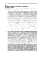
Fig. 6.1. Dependence of relative uncertainty ∆τ
0
|τ
0
upon optical thickness τ
0
with the value
of
ω
0
= 0.999. Solid lines corresponds to A = 0.7, dashed lines corresponds to A = 0.1.
1 – for reflection irradiance; 2 – for transmitted irradiance; 3 – average values
are available even for τ
0
≥ 3andtherelativeerrordoesnotexceed5%for
ω
0
≥ 0.999. The error of the retrieval of optical thickness strongly decreases
with the increasing of radiation absorption. As is shown in Fig. 6.1 the error
analysis using the numerical simulation indicates that the first formula from
(6.29) pro vides the underestimation of val ue
τ
0
for 20–50% while substituting
the reflected irradiance at the cloud top, the second one overestimates value
τ
0
,
whilesubstitutingthetransmittedirradianceatthecloudbottom,andtheav-
erage from these two values turns out to be rather close to real

τ
0
(the relative
error is about 10% for
ω
0
≥ 0.990).
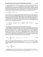
Fig. 6.2.Dependenceof relativeuncertainty ∆τ
0
|τ
0
upon ω
0
for m ean val ue of τ
0
,(6 < τ
0
< 25)
Some Possibilities of Estimating of Cloud Parameters 223
The dependence of relative error ∆τ
0
|τ
0
of the average values of the optical
thickness obtained from the reflected and transmitted irradiance assuming the
conservative scattering versus to the single scattering albedo is demonstrated
in Fig. 6.2. It is clear that the ground albedo strongly increases the uncertainty.
The interpretation of the irradiance observations within the conservative
cloud layer is available usingtheformula readily derived from (2.46) and (2.49):
– the upper sublayer adjoins the cloud top

(1 − g)
τ
1
=
4K
0
(µ
0
)−2(F
↓
1
+ F
↑
1
)
3F(τ
1
)
− q

, (6.31)
–thesublayerwithinthecloud
(1 − g)(
τ
i
− τ
i−1
) =
4(F
↓

i−1
− F
↓
i
)
3F(τ
i
)
, (6.32)
– the sublayer adjoins the cloud bottom
(1 − g)(
τ
N
− τ
N−1
) =
2(F
↓
N−1
+ F
↑
N−1
)
3F(τ
N−1
)
−

q


+
4A
3(1 − A)

, (6.33)
where N is the number of sublayers and
τ
N
= τ
0
.
6.2.2
Estimation of Phase Function Parameter g
All the above-presented expressions retrieve the scaled optical thickness, so
phase function parameter g is needed to obtain the optical thickness. The infer-
ring of phase function parameter g (asymmetry factor) of ice clouds has been
made in the 90th by measuring the radiative fluxes, calculating the radiative
transfer models, and selecting parameter g for the best coincidence with the
obser vations. However, the methodology of selecting parameters is ambiguous
as has been shown in Chap. 4 and needs careful error analysis. Probab ly, it is the
reason for inconsistent results. Besides, parameter g dramatically influences
the calculation of reflection function
ρ
∞
(µ, µ
0
), thus it has to be obtained
from measurements for the adequate interpretation of the satellite radiation
observations.
The attempts to obtain parameter g from observations has been made in

two studies (Gerber et al. 2000; Garrett et al. 2001) using the nephelometer
measurements, and the values of parameter g is revealed to be equal to 0.85
for stratiform liq uid clouds, to 0.81 for convective clouds, and to 0.73 for
nonconvective ice clouds. It is seen that the variation of the asymmetry factor
is significant and it is desirable to retrieve parameter g and the other optical
parameters together during one experiment.
Here we propose a way of estimating phase function parameter g for the
optically thick cloud from radiative observations as other o p tical parameters.
224 Analytical Method of Inverse Problem Solution for Cloudy Atmospheres
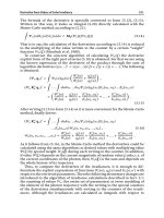
Fig. 6.3. D ependence of the ratio of K
2
(µ
0
)|[K
0
(µ
0
)g] upon solar zenith angle µ
0
;Thepoints
indicate the calculated values; the solid line is the linear approximation
Fig. 6.4. Dependence of the ratio of K
2
(µ
0
)|K
0
(µ
0
)uponthevalueofg for different µ

0
The analysis of the two-moment observation of the irradiances (two values of
solar zenith angle) indicates that the dependence of difference K
2
(µ
1
)|K
0
(µ
1
)−
K
2
(µ
2
)|K
0
(µ
2
) upon parameter g is the linear one as is shown in Fig. 6.3 for
different zenith angles (see also Fig. 6.4). Then parameter g may be empirically
expressed as follows:
g
=
1
5.57(µ
1
− µ
2
)


K
2
(µ
1
)
K
0
(µ
1
)
−
K
2
(µ
2
)
K
0
(µ
2
)

. (6.34)
Some Possibilities of Estimating of Cloud Parameters 225
However, in spite of the simplicity of (6.34), there is a problem in applying it. It
is impossible to obtain parameter g from the reflected or transmitted radiance
because the system of (6.34) with (6.11) or (6.12) for irradiance (6.13) or (6.20)
forradianceturnsouttobehomogeneous.Thereisawaytoobtainparameters
2

with another approach for example from the airborne observations with (6.1)
or (6.2). Then difference K
2
(µ
1
)|K
0
(µ
1
)−K
2
(µ
2
)|K
0
(µ
2
) is expressed through
parameter s
2
and through the observational data of the transmitted irradiance
or radiance using (6.34). Finally, parameter g is estimated using one of the
following expressions:
g
=

(ρ
0
−ρ
1

)K
0
(µ
2
)
(ρ
0
−ρ
2
)K
0
(µ
1
)
−1

[5. 57(µ
1
− µ
2
)s
2
]
g
=

σ
1
¯
K

0
(µ
2
)
σ
2
¯
K
0
(µ
1
)
−1

[5. 57(µ
1
− µ
2
)s
2
]
(6.35)
Heretheexpressionsarewrittenforthecaseoftheradianceobservational
data with demand of the horizon tal homogeneity of the cloud field. The ir-
radiance data need the temporal stability because of using the two-moment
observations, andthe formulasoftheirradiances arealmostlikewise, excluding
value F
↓
, which is substituted with value σ,and(a(µ
0

)−F
↑
), which is substi-
tuted with (
ρ
0
− ρ). The evident advantages and disadvantages are seen, while
using the reflected or transmitted radiance, or the irradiance observations.
Thus, value
ρ
∞
(µ, µ
0
) strongly depends on phase function. The dependence
of the plane albedo is weaker so using the reflected irradiance or transmit-
ted radiance is more preferable than using the reflected radiance. Using the
transmitted radiance is strongly influenced by the ground albedo, thus the
transmitted irradiance provides the better accuracy for the cloud abov e the
snow surface.
No w obtain the cloud optical parameters using the numerical model of the
radiative characteristics, calculated with the doubling and adding method.
Value s
2
and scaled optical thickness τ

are retrieved from F
↓
and F
↑
data.

Then parameter g is obtained for the pair of radiances with (6.35), and single
scattering albedo and optical thickness are calculated. Table 6.2 presents the
obtained results.
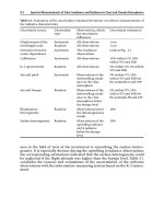
Table 6.2. Retrieval of the optical parameters of the cloud layer from the model values of the
radiative characteristics
Value Model magnitudes Retrieved magnitudes Uncertainty (%)
F
↓
0.3051
F
↑
0.6398
τ
0
25 28.55 14
ω
0
0.99900 0.99919 0.2
g 0.850 0.872 2.5
s
2
0.002222 0.002227 0.2
µ 1.0 0.846
I
↓
(µ) 0.3866 0.3499
K
0
(µ) 1.272 1.153
226 Analytical Method of Inverse Problem Solution for Cloudy Atmospheres

Even the small uncertainty of value g causes a significant error of the optical
thicknessasperexpression
τ
0
= τ

|[3(1 − g)] and is seen from Table 6.2. Model
value g
= 0.85 allows obtaining τ
0
= 24.36 with the uncertainty equal to
2.6%, while retrieved value g leads to the uncertainty equal to 14%. Hence, the
necessity of an accurate value of g is evident.
It is important to mention that a similar approach for the phase function
parameter has been considered in the book by Yanovitskij (1997) for the case
ofconservativescatteringonthebasisoftherigoroustheory.Theapproach
for obtaining parameter g hasalsobeenproposedinthestudybyKonovalov
(1997) with the approximation of the reflection function.
6.2.3
Parameterization of Cloud Horizontal Inhomogeneity
The simple appro ximate parameterization of the cloud top heterogeneity was
proposed earlier in the study by Melnikova and Minin (1977). The rough
cloud top causes an increase of the diffused radiation part in the incident
flux. Therefore, this obstacle turns out to be an essential one for calculating the
radiative characteristics dependingon solarincidentangle. Both theescape and
reflection functions describe this dependence for the reflected radiance, and
theescapefunctiontogetherwiththeplanealbedoofsemi-infiniteatmosphere
describe this dependence fo r the reflected irradiance. Thus, it was proposed
(Melnikova and Minin 1977) to replace all functions depending on incident
angle cosine

µ
0
with their modifications according to expressions:
ρ
0
(µ, µ
0
) = ρ
0
(µ, µ
0
)(1 − r)+ra(µ),
K(
µ
0
) = K(µ
0
)(1 − r)+rn ,
a(µ
0
) = a(µ
0
)(1 − r)+ra
∞
,
(6.36)
where spherical albedo a
∞
, plane albedo a(µ
0

)andvalueofn are defined with
(2.27).
a
∞
= 2
1

0
a(µ
0
)µ
0
dµ
0
= 4
1

0
µ
0
dµ
0
1

0
ρ
0
(µ, µ
0
)µdµ

n = 2
1

0
K(µ
0
)µ
0
dµ
0
(6.37)
and parameter r describes the diffused part of light in the incident flux.
The influence of the overlying atmospheric layers (including high thin
clouds), the difference between the reflection functions of the real cloud
(described by the Mie phase function) and model cloud (described by the
Henyey-Greenstein phase function), and other factors impacting the angular
dependence of radiation, are also partly corrected by parameter r.
Some Possibilities of Estimating of Cloud Parameters 227
Let us consider the numerical and analytical results concerning the cloud
heterogeneity. There have been many studies in this field lately (Tarabukhina
1987; Loeb and Davis 1997; Galinsky and Ramanathan 1998; Marshak et al.
1998). It was shown that the influence of geometrical variations of the cloud
parameters is by an order of magnitude greater than the int ernal variations
(Titov 1998). The analytical solutions (Tarabukhina 1987; Galinsky and Ra-
manathan 1998) emphasize that the cloud heterogeneity greatly impacts the
radiance and irradiance, and this obstacle is actually described with modifying
theescapefunction(ortheanalogousfunctions)aspertheexpressionsimilar
to (6.26).
There are different estimations of the role, which this impact plays, while
simulating the radiative transfer within clouds. In our case it is expressed

with the value of parameter r and the analysis of above-mentioned studies
(Tarabukhina 1987; Galinsky and Ramanathan 1998) allows us to let r ∼
0.01−0.1. Most results also show that the minimal disturbance in the radiation
field caused by the cloud heter ogeneity is at the solar angle equal to 48−49
◦
.
As has been mentioned above, all functions depending on incident angle are
approximately equal to the integrals over this angle. That is why parameter r
doesnotinfluencetheresultifthemeasurementisaccomplishedatthisincident
angle.
Parameter r can be estimated from radiance or irradiance measurements in
the stable overcast conditions with the following approach. The ground-based
and sat ellite o bservations indicat e that the measured radiance or irradiance
dependence upon solar incident angle is weaker than the dependences of the
calculated radiance andirradiance upon viewing and incidentangles (Loeb and
Davis 1997), and it is called the violation of the directional reciprocity for the
reflected radiation. Both the incident and viewing angle cosine dependences
of the radiation escaped from the optically thick layer is described with the
escape function K(
µ
0
). Thus, the data set measured during several hours could
give us the solar incident angle dependence of the escape function. If it differs
from the radiance dependence upon viewing angle, it is possible to obtain the
value of r as follows:
r
=
I(µ
1
, µ

2
)−I(µ
2
, µ
1
)
1−I(µ
1
,0.67)
K
0
(µ
1
)
K
0
(µ
1
)−K
0
(µ
2
)
. (6.38)
In this expression I(
µ
0
, µ) is the observed (reflected or transmitted) radiance.
In addition, the assumption of
ρ

0
(µ,0.67) = K
0
(0.67) = 1isusedhere.The
radiationabsorption influencing theescape function asper expression (1−3q

s)
is divided out in the ratio. Certainly, this way needs high stability of clouds
that is possible sometimes (but not often) especially in the North Regions. This
method seems preferable for ground-based observations.
There is another method for parameter r estimation from the multi-di-
rectional radiance measurements (e. g. from the measurements by POLDER
instrument). The approximate values of the optical thickness of the cloud layer
are obtained for every available viewing direction and for every pixel assuming
the conservative scattering at the first stage of data processing and (2.24). Then
228 Analytical Method of Inverse Problem Solution for Cloudy Atmospheres
theaveragevalueoftheopticalthicknessiscalculatedforeverypixel.The
relative deviations of the optical thickness obtained for every direction from
the average one could be taken as a measure of the deviation of the cloud top
from the plane. It is necessary to have in mind that parameter r also includes
the influence of the radiation scattering by the above atmospheric layers and
thin semitransparent above clouds. Then the following is proposed for the
evaluation of parameter r:
r
=
1
N
¯
τ
N


i=1
|
¯
τ − τ
i
| , (6.39)
where N is the number of viewing directions for every pixel and
¯
τ is the average
optical thickness over viewing directions. This methodology was applied to
POLDER (Polarization and Directionality of the Earth’s Reflectance) Level-2
data containing the reflected radiance at 14 directions (Melnikova and Naka-
jima 2000).
6.3
Analysis of Correctness and Stability of the Inverse Problem Solution
The above-proposed set of formulas is the solution of the inverse problem of
atmospheric optics for the accepted cloud model. According to the book by
Prasolov (1995) the range of the continuality of the obtained functions is to be
analyzed for testing the solution correctness.
In the case of (6.1) the analysis of continuality and positiveness of function
s
2
(F
↓
, F
↑
, µ
0
) taking into account evident condition F(0) ≥ F(τ

0
)yieldsthe
following inequalities:
– For cosine of solar incident angle
µ
0
> 0.3
1 > 2[F
↑2
(0) + F
↓2
(τ
0
)−F
↓
(τ
0
)F
↑
(τ
0
)] + F(0) ,
s[8.0 + 0.2(1 − A)] > 0.54(1 − A)
2
+0.3(1−A),
(6.40)
– For cosine of solar incident angle
µ
0
> 0.9

1 > 0.7[F
↑2
(0) + F
↓2
(τ
0
)−0.7F
↓
(τ
0
)F
↑
(τ
0
)] + 1.1F(0) ,
s[8.0 − 0.2(1 − A)] > 0.54(1 − A)
2
−0.2(1−A).
(6.41)
The concrete numerical magnitudes of the parameters providing continuality
and positiveness of function s
2
(F
↓
, F
↑
, µ
0
) are different for ever y observed pair
of upwelling and down welling irradiances at the single level and wavelength.

Thus, the experimental data have to be tested for satisfying these inequalities
before applying (6.1) to the observational results. Corresponding procedures
are provided in the algorithms of the observational data processing. The anal-
ogous inequality could be easily derived for all cases considered hereinbefore
andthecorrespondinganalysisisincludedtotheprocessingalgorithms.
Analysis of Correctness and Stability of the Inverse Problem Solution 229
6.3.1
Uncertainties of Derived Formulas
There are four main sources of uncertainties, while using the proposed formu-
las for the retrieval of the cloud optical parameters:
1. observational uncertainties;
2. a priori specification of parameter g;
3. breakdown of the applicability region of the asympto tic formulas;
4. inhomogeneity of the cloud layer, while the derived expressions are as-
suming the cloud homogeneity (while consideration of the observations
within the cloud layer).
I t is easy to deduce the corresponding formulas for relative uncertainties
∆s|s
and
∆τ
0
|τ
0
caused by observational uncertainty, as we have the analytical
expressions for the calculation of the optical parameters using the approach
described in Sect. 4.3, namely, if the vector of observations y
= f (x
1
, x
2

, ,x
n
),
then:
∆y ≤




∂f
∂x
1




∆x
1
+




∂f
∂x
2





∆x
2
+ +




∂f
∂x
n




∆x
n
,
where
∆x
i
isthemeansquaredeviationcausedbytheobservationaluncertainty
or interpolation of the functions over look-up tables.
In particular, if irradiances F
↑
and F
↓
have been measured with uncertainty
∆F and the optical parameters have been calculated with (6.1), the expression
of the relative uncertainties are the following (Melnikova 1992; Melnikova and
Mikhailov 1994):

∆s
s
≤
∆F
1−F
↑
− F
↓
+
2
∆Fa
2
(µ
0
)+16K
0
(µ
0
)∆K
0
+ F(0)∆a
2
16K
0
(µ
0
)−2F(0)a
2
(µ
0

)
, (6.42)
and for relative uncertainty
∆τ
0
|τ
0
:
∆τ
0
τ
0
≤
1
τ
0

30∆s +
∆F
F(0)
2

+
∆g
1−g
+
∆s
s
, (6.43)
where value 1 − F

↑
− F
↓
defines the radiative flux divergence in the cloud layer
in relative units
πS. In the short-wave range it is about 0.05–0.2. Then the first
item provides the order of the magnitude of the uncertainty, namely
∆s|s ≥ 4%
for
∆F ∼1–3W|m
2
.
The uncertainties of functions
∆K
0
(µ
0
)and∆a
2
(µ
0
)areinducedfortwo
reasons: the inaccurat e measuring of the incident angle and the income of
partly scattered solar radiation to the cloud top. The first reason (measuring
of solar incident angle arccos
µ
0
)couldnotgiveasignificanterrorasthevalue
of
µ

0
is defined by the moment and geographical site of the observation and
230 Analytical Method of Inverse Problem Solution for Cloudy Atmospheres
these parameters are known with sufficient accuracy. Concerning the second
reason, we present the following consideration. Ac cording to the book by Minin
(1988), the part of diffused radiation in the clo udless atmosphere de pends on
solar incident angle and wavelength, and this part is approximately equal to
0.3 of the total flux. Function K
0
(µ
0
)transformstovaluen and function a
2
(µ
0
)
transforms to value 12q

= 8.5 for the fully diffused radiation, that yields
∆K
0
∼ 0.03 and ∆a
2
∼ 0.25, and these values are minimal for µ
0
= 0.6−0.7.
This condition should be provided during observations.
Relative uncertainty
∆τ
0

|τ
0
is defined mainly by uncertainties of the retrieval
∆s|s and ∆g|(1 − g) as per (6.43), because the first item could be rather small
in the case of large cloud optical thickness and could weakly influence the
uncertainty. The value of
∆g|(1 − g) is caused by the second uncertainty source
and it depends on the consistency of the model value of parameter g to the real
cloud property. In accordance with the results of the study by Stephens (1979)
where the spectral values of g have been calculated with Mie theory for eight
cloud models, assuming g
= 0.85, it is possible to conclude that the variation s
of parameter g in the short wavelength region are not exceeding 2%.
Uncertainty
∆s|s provided by (6.3)–(6.5) yields ∆s|s ≤ 0.05 after calculating
the corresponding derivatives and substituting
∆F ∼ 1−3W|m
2
.Therelative
uncertainty of single scattering albedo
ω
0
is derived from expression 1 − ω
0
=
3s
2
(1 − g):
∆(1 − ω
0

)|(1 − ω
0
) = 2∆s|s + ∆
g
|(1 − g) . (6.44)
Assuming value s ≤ 0.05, we have:
∆(1 − ω
0
)|(1 − ω
0
) ≤ 0.12.
Relative uncertainty
∆τ
0
|τ
0
provided b y (6.6)–(6.8) is estimated according
to the following expression (Melnikova and Mikhailov 2001):
∆τ
0
|τ
0
∼ 2∆F


∆s(F
↓
− F
↑
)(1 − g)


+ ∆s|s + ∆g|(1 − g) . (6.45)
Thevaluesofthetwofirstitemsinthesumdefinedbytheobservational
uncertainty and by the uncertainty of the retrieval of parameter s is about 15%,
the third item adds 2%, thus
∆τ
0
|τ
0
∼ 17%.
The error analysis in the case of using the reflected or transmitted irradiance
with (6.11) and(6.12)shows that the temporal stability of the cloud layer during
observations is necessary. As has been demonstrated in Sect. 1.5, the existence
of the overcast cloudiness during one hour is rather probable (about 80%).
Uncertainties
∆s|s and ∆τ
0
|τ
0
are calculated in the case of using the reflected
irradiance by the following expressions:
∆s
s
=
∆
K
0
(a − F
↑
)+K

0
(µ
2
)(∆a + ∆F)
K
0
(µ
2
)(a(µ
1
)−F
↑
1
)−K
0
(µ
1
)(a(µ
2
)−F
↑
2
)
+
∆K
0
(a − F
↑
)+K
0

(∆a + ∆F)
2K
0
(µ
11
)(a(µ
2
)−F
↑
2
)
+
2
∆w(µ
1
)+∆n
2
(w(µ
1
)−w(µ
2
))n
2
(6.46)
Analysis of Correctness and Stability of the Inverse Problem Solution 231
∆τ
0
τ
0
=

∆
s
s
+

∆
¯
l
¯
l
+
mnK(
µ)(
∆m
m
+
∆n
n
+
∆K
K
)+∆l(a(µ)−F
↑
)+l(∆a − ∆F
↑
)
mnK(µ)+l(a(µ)−F
↑
)
+

∆a − ∆F
↑
a(µ)−F
↑

1
τ
0
.
And in case of using the transmitted irradiance:
∆s
s
=
2∆w + ∆n
2
(w(µ
1
)−w(µ
2
))Q
2
+
∆FK
0
+ ∆K
0
F
↓
F
↓

1
K
0
(µ
2
)−F
↓
2
K
0
(µ
1
)
+
∆FK
0
(µ
1
)+∆K
0
F
↓
2F
↓
2
K
0
(µ
1
)

,
(6.47)
∆τ
0
τ
0
=
∆
s
s
+
⎡
⎢
⎣
∆r
r
+
r
2
l
¯
l

∆l
l
+
∆
¯
l
¯

l
+
2∆r
r



1+
r
2
l
¯
l
+1

2

1+
r
2
l
¯
l
⎤
⎥
⎦
1
τ
0
,

where
∆r
r
=
∆
F
F
+
∆m
m
+
∆¯n
¯n
+
∆K
K
+
∆l
l
+
∆
¯
l
¯
l
.
The error analysis as per (6.46)–(6.47) gives ∆s|s ∼ 8% and ∆τ
0
|τ
0

∼ 10% for
reflected irradiance and for transmitted irradiance – 6% and 10% correspond-
ingly, if the observation al uncertainty is about 2%. In general, the irradiances
data allow obtaining the optical parameters within the cloud more accurately
than the radiances do, according to the study by McCormick and Leathers
(1996).
6.3.2
The Applicability Region
As has been mentioned in Sect. 2.4, the main lower bound connecting with the
diffusion domain is set on the optical thickness. The restriction on the true
absorption arises due to expansions o ver the small parameter for the asymp-
totic constants. The applicability region of the inverse expressions for values s
and
τ

have been studied in several studies (Melnikova 1992, 1998; Melnikova
et al. 2000) for the wide set of parameters. Calculation of the direct problem
has been accomplished with the doubling and adding method, and the ob-
tained radiative characteristics have served as measured values (Demyanikov
and Melnikova 1986). The retrieved parameters have been compared with the
model parameters of the direct problem for estimating the relative error. About
50 numerical models have been analyzed in total. The values of the relativ e un-
certainties of 1−
ω
0
and τ
0
with fixed phase function parameter g are presented
in Figs. 6.5 and 6.6 versus the single scattering albedo and optical thickness
correspondingly. We should point out that the only uncertainties caused by the

break of the applicability region have been studied in the above-mentioned
232 Analytical Method of Inverse Problem Solution for Cloudy Atmospheres
Fig. 6.5.Relative uncertainties ∆τ
0
|τ
0
(solid line)andg∆(1−ω
0
)|(1−ω
0
)(dashed line)versus
value
ω
0
with fixed value τ
0
= 25
Fig. 6.6. Relative uncertainties ∆(1 −ω
0
)|(1 −ω
0
)(solid line)and∆τ
0
|τ
0
(dashed line)versus
value
τ
0
with fixed value ω

0
= 0.999
analysis, and the values of the radiative characteristics have been assumed as
the exact ones.
The radiative characteristics of the inhomogeneous cloud layer have been
calculated with the doubling and adding method for five sublayers with optical
thickness
τ
i
= 5 and single scattering albedo ω
0,i
together with asymmetry
factor g (two latter parameters varying for sublayers). The irradiances have
been calculated at the boundaries of sublayers. Then the optical parameters
have been retrieved with formulas (6.11) and (6.12). Table 6.3 demonstrates
the obtained results and the uncertainties of these results. The results of the
References 233
Table 6.3. Influence of the vertical heterogeneity of the layer on the exactness of the optical
parameters retrieval
iG ω
0
τ

model
s
2
model
τ

s

2
∆s
2
(%) ∆τ

(%)
Inhomogeneous la y ers
1 0.85 0.999 2.25 0.00222 2.29 0.00235 4.0 4.8
2 0.85 0.999 2.25 0.02222 2.27 0.02287 2.7 3.6
3 0.85 0.970 2.25 0.06667 2.17 0.07042 5.8 5.2
4 0.85 0.950 2.25 0.10870 2.54 0.11620 7.3 9.4
5 0.85 0.930 2.25 0.15556 2.95 0.15732 8.8 15
Homogeneous layers
1 0.85 0.999 4.59 0.00222 4.72 0.00228 3.0 3.1
3 0.85 0.970 4.59 0.06667 4.80 0.06349 5.4 5.0
analysisfortwocasesofthehomogeneouslayerswithcorrespondingvaluesof
τ
0
and ω
0
are presented in the same table.
As isseen from thetable,theuncertainty in thecase ofinhomogeneous layers
is the same as in the case of the homogeneous layers and depends only on the
applicability region of the used equations (magnitudes of the single scattering
albedo and optical thickness). The high values of the uncertainties appear only
for the high absorbing sublayers with values of the single scattering albedo
ω
0,i
= 0.95 and 0.93, which provide significant errors both for the irradiance
calculation (Fig. 2.2) and for the retrieved parameters (Fig. 6.5).

References
Boucher O (1998) On aerosol direct forcing and the Henyey-Greenstein phase function.
J Atmos Sci 55:128–134
Demyanikov AI, Melnikova IN (1986) On the applicability region determination for asymp-
totic formulas of monochromatic radiation transfer theory. Izv Acad Sci USSR. Atmo-
sphere and Ocean Physics 22:652–655 (Bilingual)
Dlugach JM, Yanovitskij EG (1974) The optical properties of Venus and Jovian planets. II.
Methodsandresultsofcalculationsoftheintensityofradiationdiffuselyreflectedfrom
semi-infinite homogeneous atmospheres. Icarus 22:66–81
Duracz T, McCormick NJ (1986) Equation for Estimating the Similarity P arameter from
Radiation M easurements within Weakly Absorbing Optically Thick Clouds. J Atmos Sci
43:486–492
Galinsky VL, Ramanathan V (1998) 3D Radiative transfer in weakly inhomogeneous
medium. Part I: Diffusive approximation. J Atmos Sci 55:2946–2955
Garret T, Hobbs PV, Gerber H (2001) Shortwave, single scattering properties of arctic ice
clouds. J Geoph Res 106(D14):15155–15172
Gerber H, Takano Y, Garret T, Hobbs PV (2000) Nephelometer measurements of the asym-
metry parameter, volume extinction coefficient, and backscatter ratio in arctic clouds.
J Atmos Sci 57:2320–2344
234 References
Germogenova TA, Konovalov NV, Lukashevitch NL, F eigelson EM (1977) Im proval of the
interpretation of optical observations from the board of automa tic interspace station
“Venera-8”. Cosmic studies, XV: Iss 5. (in Russian)
Ivanov VV (1976) Radiative transfer in multi-layered optically thick atmosphere. Studies of
the Astronomical Observatory (Mathematical Sci) Leningrad 32:3–23 (in Russian)
King MD (1983) Number of terms required in the Fourier expansion of the reflection
function for optically thick atmospheres. J Quant Spectrosc Radiat Transfer 30:143–161
King MD (1987) Determination of the scaled optical thickness of cloud from reflected solar
radiation measurements. J Atmos Sci 44:1734–1751
King MD (1993) Radiative pro perties of clouds. In: Hobbs V (ed) Aerosol-cloud-climate

interactions. Academic Press, New York, pp 123–149
King MD, Radk e L, Hobbs PV (1990) Determination of the spectral absorption of solar
radiation by marine stratocumulus clouds from airborne measurements within clouds.
J Atmos Sci 47:894–907
Kokhanovsky A (1998) Variability of the phase function of atmospheric aerosols at large
scattering angles. J Atmos Sci 55:314–320
Kokhanovsky A, Nakajima T, Zege E (1998) Physically based parameterizations of the
short-wave radiative characteristics of weakly absorbing optically media: application to
liquid-water clouds. Appl Opt 37:335–342
Kokhanovsky AA,RozanovVV,Zege EP, Boven smannH, Burrows JP (2003)A semianalytical
cloud retrieval algorithm using backscattered radiation in 0.4–2.4
µmspectralregion.J
Geophys Res 108(D1,4008,doi:10.1029/2001JD001543)
Konovalov NV (1982) Asymptotic properties of the transfer equation solution in plane-
parallel layers. PhD Thesis, (KIAM) RAS, Moscow (in Russian)
Konovalov NV (1997) Certain properties of the reflection function of optically dense la y-
ers. Preprint of Keldysh Institut e for Applied Mathematics (KIAM) RAS, Moscow (in
Russian)
Konovalov NV, Lukashevitch NL (1981) The inverse problem of the interpretation of optical
observations within the Venus atmosphere from the station “Venera-10”. Preprint of
Keldysh Institute for Applied Mathematics (KIAM) RAS, Iss 15 Moscow (in Russian)
Loeb NG, Davies R (1997) Angular dependence of observed reflectance: a comparison with
plane parallel theory. J Geophys Res 102:6865–6881
Marshak A, Davis A, Wiscomb W, Cahalan R (1998) Radiativ e effects of sub-mean free path
liquid water variability observed in stratiform clouds. J Geoph Res 103(D16):19557–
19567
McCormick NJ, Leathers RA (1996) Radiative Transfer in the Near-Asymptotic Regime. In:
IRS’96: Current Problems in Atmospheric Radiation:826–829
Melnikova IN (1991) Spectral coefficients of scattering and absorption in strati clouds.
Atmospheric Optics 4:25–32 (Bilingual)

Melnikova IN (1992a) Analytical formulas fo r obtaining optical parameters of cloud layer
from measured characteristics of solar radiation field. I. Theory. Atmosphere and Ocean
Optics 5:169–177 (Bilingual)
Melnikova IN (1998) Vertical profile of spectral scattering and absorption coefficients of
stratus clouds. I. Theory. Atmospheric and Ocean Optics 11:5–11 (Bilingual)
Melnikova IN, Minin IN (1977) To the transfer theory of monochromatic radiation in cloud
layers. Izv Acad Sci USSR Atmosphere and Ocean Physics 13:254–263 (Bilingual)
Melnikova IN, Mikhailov VV (1993) Obtaining of optical characteristics of cloud layers.
Doklady of Russian Academy of Sciences 328:319–321 (Bilingual)
References 235
Melnikova IN, Mikhailov VV (1994) Spectral scattering and absorption coefficients in strati
derived from aircraft measurements. J Atmos Sci 51:925–931
Melnikova IN, Fedorova EYu (1996) Vertical profile of optical parameters inside cloud layer.
In: Problems of Atmospheric Physics, St.Petersburg State University Press, St.Petersburg
6:261–272 (in Russian)
Melnikova IN, Zshanabaeva SS (1996) Evaluation of uncertainty of approximate method-
ology of accounting the vertical stratus structure in direct and inverse problems
of atmospheric optics. International Aerosol Conference, December, Moscow (in
Russian)
Melnikov a IN, Zshanabaeva SS (1996) Exactness of method for calculation of solar irra-
diances in vert ical inhomogeneous scattering layers. Intern Symp “Geokosmos”, June,
St.Petersburg (in Russian)
Melnikov a IN, Domnin PI (1997) Determination of optical parameters of homogeneous
optically thick cloud layer. Atmosphere and Ocean Optics 10:734–740 (Bilingual)
Melnikov a IN, Nakajima T (2000) Single scattering albedo and optical thickness of stratus
clouds obtained from “POLDER” measurements of reflected radiation. Earth Observa-
tions and Remote Sensing 3:1–16 (Bilingual)
Melnikova IN, Solovjeva SV (2000) Solution of direct and inverse problem in case of cloud
layers of arbitrary optical thickness and quasi-conservative scattering. In: Ivlev LS (ed)
Natural and anthropogenic aerosols, St. Petersburg, pp 86–90 (in Russian)

MelnikovaIN, MikhailovVV (2001) Vertical profiles ofstratusclouds spectral optical param-
eters derived from airborne radiation measurements. J Geophys Res 106(D21):27465–
27471
Melnikova IN, Domnin PI, Radionov VF (1998) Retrieval of optical thickness and single
scattering albedo from measurements of reflected or transmitted solar radiation. Izv
RAS Atmosphere and Ocean Physics 34:669–676 (Bilingual)
Melnikova IN, Dlugach ZhM, Nakajima T, Kawamoto K (2000) On reflected function calcu-
lation simplification in case of cloud layers. Appl Optics 39:541–551
Melnikova IN, Domnin PI, Radionov VF, Mikhailov VV (2000) Optical characteristics of
clouds derived from measurements of reflected or transmitted solar radiation. J Atmos
Sci 57:623–630
Minin IN (1988) The theory of the radiation transfer in the planets atmospheres. Nauka,
Moscow (in Russian)
Minin IN, Tarabukhina IM (1990) To studying of optical properties of the Venus atmosphere
(Bilingual). Izv Acad Sci USSR Atmosphere and Ocean Physics 26:837–840
Prasolov AV (1995) Analytical and numerical methods of dynamic processes studying. St.
Petersburg State University Press, St. Petersburg (in Russian)
Rozenberg GV, Malkevitch MS, Malkova VS, Syachinov VI (1974) Determination of the
optical characteristics of clouds from measurements of reflected solar radiation on the
Kosmos-320 satellite. Izv. Acad. Sci. USSR. Atmosphere and Ocean Physics 10:14–24 (in
Russian)
Stephens GL (1979) Optical properties of eight water cloud types. Technical Paper of CSIRO,
Atmos Phys Division, Aspendale, Australia, No. 36:1–35
Tarabukhina IM (1987) On the reflection and transmission of light by a horizontally inho-
mogeneous optically thick layer. Izv RAS, Atmosphere and Ocean Physics 23:148–155
(Bilingual)
Titov GA (1998) Radiative horizontal transport and absorption in stratocumulus clouds. J
Atmos Sci 55:549–2560
236 References
Ustinov EA (1977) The inverse problem of the multiple scattering theory and interpretation

of the diffused radiation observations within the Venus atmosphere. Space Studies
15:768–775 (in Russian)
Van de Hulst HC (1980) Multiple Light Scattering. Tables, Formulas and Applications, Vol.
1 and 2. Academic Press, New York
Yanovitskij EG (1972) Spherical albedo of planet atmosphere. Astronomical J 49:844–849
(in Russian)
Yanovitskij EG (1997) Light scattering in inhomogeneous atmospheres. Springer, Berlin
Heidelberg New York
Zege EP, K okhanovsky AA (1994) Analytical solution for optical transfer function of a light
scattering medium with large particles. Applied Optics 33:6547–6554
CHAPTER 7
Analysis of Radiative Observations
in Cloudy Atmosphere
7.1
Optical Parameters of Stratus Cloudiness Retrieved
from Airborne Radiative Experiments
The data of airborne experiments accomplished in 1970–1980-th within the
range of research programs CAENEX, GATE, GARP have been presented in
Sect. 3.3 with the results of the experiments under the overcast conditions
being listed in Table 3.2. These results are used here for inferring spectral
dependence of the optical parameters of cloud layers (optical thickness
τ
0
and single scattering albedo ω
0
), applying the approach described in Chap. 6
(Melnikova 1989, 1992; Melnikova and Mikhailov 1993,1992). The spectral
values o f phase function parameter g, needed for obtaining optical thickness
τ
0

,
single scattering albedo
ω
0
, and the volume scattering coefficient are taken
from the study by Stephens (1979). The procedure of retrieval is presented in
detail elsewhere (Melnikova 1992, 1997; Melnikova and Mikhailov 1994).
7.1.1
Analysis of the Results of Radiation Observations in the Tropics
The observations were carried out as a part of the GATE experiment above the
Atlantic Ocean close to the west coast of Africa (experiment No. 1: 12th July
1974, the latitude was 16
◦
N, experiment No. 2: 4th August 1974, the latitude
was 17
◦
N). The cloud bottom and top were at altitudes 0.3–3.3 and 0.5–5.0 km
for experiments 1 and 2 correspondingly. The uncertainties of the observations
were abou t 5–7% depending on wavelength. The retrieval of the optical param-
eters was implemented for every wavelength independently using (6.1). The
spectral values of optical thickness
τ
0
and single scattering co-albedo (1 − ω
0
)
are shown in Figs. 7.1a and 7.2a correspondingly and the volume absorption
and scattering coefficients are shown in Table A.12 of Appendix A. The oscil-
lation s in the curves presenting the optical thickness in Fig. 7.1a are explained
with the high observational uncertainties; the smoothed curves are figured

there as well. It should be mentioned that the high values of single scattering
co-albedo (1 −
ω
0
) are explained with the strong flue sand escaping from the
Sahara Desert to the observational site.
238 Analysis of Radiative Observations in Cloudy Atmosphere
Fig. 7.1a–d. Spectral dependence of optical thickness τ
0
retrieved from the data of airborne
radiative observations for different latitudinal zones: a 17
◦
N; b 45
◦
N; c 60
◦
N; d 75
◦
N