- Trang chủ >>
- Khoa Học Tự Nhiên >>
- Vật lý
Green Energy Technology, Economics and Policy Part 8 ppt
Bạn đang xem bản rút gọn của tài liệu. Xem và tải ngay bản đầy đủ của tài liệu tại đây (218.65 KB, 35 trang )
230 Green Energy Technology, Economics and Policy
Demonstration The technology is demonstrated in practice. Costs are high.
External (including government) funding may be needed to
finance part or all of the costs of demonstration.
↓
Deployment Successful technical operation, but possibly in need of support
to overcome cost or non-cost barriers. With increasing
deployment, technology learning will progressively decrease
costs.
↓
Commercialization The technology is cost competitive in some or all markets,
(diffusion) either on its own terms, or where necessary, supported by
government intervention (e.g. to value externalities, such as
costs of pollution).’’
On the demand side, economically-viable technologies which are capable of delivering
two-thirds of the needed reduction in CO
2
emissions, already exist. The commercial-
ization of technologies that are needed for the abatement of the remaining one-third of
CO
2
emissions, cannot take place without the support of the government. Though the
technologies are cost effective, they have not penetrated the market, as the consumers
tend to take a short-term view of costs rather than a long-term life-cycle costs. For
example, a filament lamp is cheaper to buy than a fluorescent lamp to start with, but
a fluorescent lamp is cheaper in terms of the life-cycle costs because of its lower elec-
tricity consumption. Governments may promote the penetration of such technologies
through appropriate regulations.
On the supply side, CCS (Carbon dioxide Capture and Storage) and supercritical
and ultra-supercritical technologies are expensive. They can become competitive only
when a value is attached to the reduction of CO
2
emissions (say, $ 50/t CO
2
). Govern-
ments have to identify suitable technological mechanisms and design and implement
appropriate policy instruments to remove market and non-market barriers to diffusion.
18.2 TECHNOLOGY LEARNING CURVES
Generally, new energy technologies tend to be more expensive than incumbent tech-
nologies. Technology learning is the process by which the costs of the new technologies
are brought down, through reduction in production costs and improved technical
performance. The rate at which consumers switch from old to new technologies will
depend upon the relative costs and the value that the consumers attach to the long-term
life-cycle costs.
When the private industry finds that a given technological process has a good market
potential, they may perform appropriate R&D to make it marketable (“learning-by-
searching’’), or they may improve the manufacturing process (“learning-by-doing),
or the product may be modified on the basis of the feedback from the consumers
(“learning-by-using’’). The more a technology is adapted, the more will be the
improvement in technology.
Technology learning has an important role to play in R&D and investment decisions
in respect of emerging technologies. Technology learning curves may be made use of to
Deployment and role of technology learning 231
Cumulative installed capacity
Baseline
Deployment
cost
Cost of
clean technology
BLUE
Unit cost
ACT
Cumulative investment cost of
incumbent technology
Learning investments
Break-even with
CO
2
price
Break-even point
Cost of
incumbent
technology
Figure 18.1 Learning curves, deployment costs and learning investments
(Source: EnergyTechnology Perspectives, 2008, p. 204, © IEA – OECD)
estimate the deployment and diffusion costs of new technologies. Governments could
make use of this information for decision-making in regard to technology and policy
options about new energy systems.
As production doubles, the investment costs decrease. Based on this relationship,
it is possible to estimate the deployment costs of the new technologies. In the graph
between the cumulative installed capacity and the deployment cost per unit, the blue
line (learning curve) depicts the reduction in the cost of new technology as the cumu-
lative capacity increases. The grey line represents the cost of the incumbent fossil fuel
technology. The break-even point occurs when the cost of clean (new) technology
equals the cost of the incumbent fossil fuel technology. (Fig. 18.1 Schematic repre-
sentation of learning curves, deployment costs and the learning investments. Source:
Energy Technology Perspectives, 2008, p. 204).
Deployment costs for making the new technology competitive, are the sum total of
incumbent technology costs (yellow rectangle) and the additional costs needed for the
new technology to reach the break-even point (orange triangle).
In Fig. 18.1, the line representing ACT map scenario is indicative of the carbon
prices of USD 50/t CO
2
, and the line representing BLUE map scenario is indicative of
the carbon prices at USD 200/t CO
2
. Thus, the higher the carbon penalty, the higher
would be the cost of the incumbent fossil fuel technology, and the lower would be the
learning costs.
Though the learning curves have been constructed for a number of supply-side
technologies, demand-side technologies also figure in the learning curves.
The limitations of the learning curves need to be kept in mind when using them to
make investment decisions:
• The learning curves are based on price, rather than cost data.
• The factors that will drive the future cost reductions may be different from those
of the past.
• The cost of bringing energy-efficient appliances to the market should take into
account not only the bottom-up engineering models (which tend to overestimate
232 Green Energy Technology, Economics and Policy
Table 18.1 Gives the observed training rates for various electricity supply technologies (the data mostly
refers to OECD countries).
Learning
Technology Period rate (%) Performance measure
Nuclear 1975–1993 5.8 Electricity production cost (USD/kWh)
Onshore wind 1982–1997 8 Price of the wind turbine (USD/kW)
1980–1995 18 Electricity production cost (USD / kWh)
Offshore wind 1991–2006 3 Installation cost of wind farms (USD/kW)
Photovoltaics (PV) 1976–1996 21 Price of PV module (USD/W peak)
1992–2001 22 Price of balance of system costs
Biomass 1980–1995 15 Electricity production cost (USD /kWh)
Combined heat and 1990–2002 9 Electricity production cost (USD/kWh)
power (CHP)
CO
2
capture and 3–5 Electricity production cost (USD/kWh)
storage (CCS)
(Source: EnergyTechnology Perspectives, 2008, p. 205)
costs as they are based on the higher costs of more efficient components), but also
the impact of “learning-by-doing’’ which tend to reduce the costs.
• Most technologies spill over national boundaries, and hence global learning rates
would be more meaningful. Where learning occurs locally (for instance, photo-
voltaic installations in tropical countries), national learning costs would be more
relevant.
• Learning curves may be affected by changes in technology regimes resulting from
government regulations, and changes in the design of devices. The learning curve
rate may be affected depending upon the starting year from which data has been
collected.
• Learning curve rates are also affected by supply-chain effects, such as, shortage
of silicon in PV industry, steel for making wind turbines, and reactor vessels in
the nuclear industry. This led to innovations, such as Cd-Te/thin-film technologies
in PV industry, and 10 MW wind power generators using blades of light-weight
materials, and avoiding gear boxes, in the case of wind power installations.
In sum, it is important to remember that the learning curves are not set in stone, but
are subject to change as the processes underlying them, change.
18.3 COMMERCIALIZAT ION OF POWER GENERATION
T ECHNOLOGIES
Modeling technology deployment costs on the basis of learning rates is not easy – if a
low pessimistic learning rate is assumed for a technology, it may be squeezed out by
technologies with higher learning rate; if a highly optimistic learning rate is assumed,
it may lead to unrealistically high estimates of potential cost reductions.
The International Energy Agency (IEA) camp up with estimated commercialization
costs of power generation technologies, based on reasonable learning rates (Table 18.2)
234 Green Energy Technology, Economics and Policy
raise the cost of the incumbent fossil technology and would make the new technology
competitive at a lower level of deployment. For instance, a USD 50/t CO
2
incentive
would lead to 63% reduction in deployment costs for cleaner energy technologies
during 2005 to 2050, for buildings, transport and industry (from USD 1.6 trillion to
USD 0.6 trillion), and 45% reduction for power generation (from USD 3.2 trillion to
USD 1.8 trillion). A USD 200/t CO
2
incentive under the BLUE map scenario has not
been analyzed by IEA in detail as it is highly uncertain whether it would be possible
to implement it.
It would be instructive to estimate the breakdown of the deployment costs for power
generation for Baseline, ACT and BLUE map scenarios for the periods, 2005 to 2030
and from 2030 to 2050. A significantly higher investments are needed for wind, solar
thermal, nuclear Generation III and Generation IV and CCS technologies, for ACT
scenarios than for Baseline scenarios. The difference between ACT and BLUE map
scenarios is minor, and is attributed to higher investment costs for tidal and geothermal
technologies under BLUE map scenario.
On the Demand side, hybrid vehicles and solar heating account for the largest share
of deployment costs in 2005–2030 period, while the CCS industry is expected to
dominate the 2030–2050 period.
18.5 REGIONAL DEPLOYMENT FOR KEY POWER GENERATION
TECHNOLOGIES
As should be expected, the projected rate of diffusion of new technologies varies from
country to country, depending upon the present position of diffusion and capacity for
technology exploitation. The key players are expected to be USA and China.
Onshore wind: Electricity from onshore wind is already competitive with fossil
fuel energy at selected sites. It will be competitive globally by about 2020, when the
cumulative global capacity reaches 650 GW. Western Europe currently dominates the
onshore wind. USA and China will pick up rapidly after 2020. USA is expected to reach
a capacity of 200 GW by 2025. China will reach onshore wind power of 250 GW by
2040.
Table 18.4 Regional deployment of power generation technologies
Wind Photovoltaics CCS* Nuclear
2005 2030 2005 2035 2030 2050 2005 2020 2050
OECD North America 13% 24% 27% 25% 35% 25% 34% 31% 27%
OECD Europe 69% 34% 19.5% 25% 35% 16% 32% 25% 15%
OECD Pacific 2% 10% 51.7% 30% 10% 5% 17% 17% 14%
China 3% 21% 0.0% 10% 12% 33% 2% 8% 23%
India 5% 4% 0.2% 5% 3% 10% 1% 3% 7%
Others 6% 7% 1.7% 5% 5% 11% 14% 15% 14%
*CCS – Carbon dioxide Capture and Storage
(Source: ETP 2008, p. 212)
Deployment and role of technology learning 235
Offshore wind: Western Europe currently accounts for 93% of offshore wind instal-
lations in the world. This technology is expected to reach commercialization between
2035 and 2040, when it is expected to reach 250 GW. High costs of offshore wind are
a barrier for its spreading.
Photovoltaics (PV): Japan leads the world in PV technology. The PV capacity of
Japan is 2.8 GW, which is 47% of the global capacity. Western Europe and USA are
the other major centres. It is expected that during 2030–2040, the costs of deployment
of PV will become competitive. By 2045, USA will account for 50% of the global
capacity of 545 GW.
CCS: A carbon incentive of USD 50/t CO
2
is needed to facilitate the widespread
adoption of CCS. Under the ACT Map scenario, CCS deployment is expected to begin
in 2020 when USA will have the largest share of CCS deployment. By 2050, China
will dominate the CCS field globally, with significant capacities in Canada and India.
Nuclear: Significant deployment of Generation III+ and Generation IV nuclear tech-
nologies is expected to take place in Canada and USA, China and India, Russia and
western Europe and Japan. High investment costs, concerns about reactor safety, dis-
posal of nuclear wastes and nuclear proliferation, scarcity of highly skilled manpower,
are impeding the growth of nuclear power. IEA estimates that Generation III+ tech-
nologies will continue to be deployed until 2020 to 2030. After 2030, the focus will
be on Generation IV technologies.
18.6 BARRIERS TO TECHNOLOGY DIFFUSION
ETP 2008, p. 215, elucidated different issues involved in technology diffusion.
The rate of technology diffusion depends upon the following market characteristics
for individual products: (i) rate of growth of the market, and the rate at which the
old capital stock is phased out, (ii) the rate at which new technology can become
operational, (iii) the availability of a supporting infrastructure, and (iv) the viability
and competitiveness of alternative technologies. Other factors that have a bearing on
the rate of diffusion are: government policy in phasing out of constraining standards
and regulations, and introduction of new technologies, availability of skilled personnel
to produce, install and maintain new equipment, ability of the existing suppliers to
market new equipment, dissemination to the consumers of concerned information, and
incentives for buying, of new equipment, and extent of compliance with regulations
and standards.
Rapid diffusion of technology needs the removal of the following barriers: (i)
Investors are not induced to invest due to the non-availability of clear and persua-
sive information about a product, (ii) Transaction costs (i.e. indirect costs of a decision
to purchase and use equipment) are high, (iii) Buyer perceives a risk higher than it
actually is, (iv) Costs of alternative technologies are not correctly estimated, and mar-
ket access to funds is difficult, (v) High sunk costs, and tax rules that favour long
depreciation periods, (vi) Excessive/inefficient regulation which does not keep pace
with emerging situation, (vii) Inadequate capacity to introduce and manage new tech-
nology, and (viii) Non-realisation of the benefits of economy of scale and technology
learning.
236 Green Energy Technology, Economics and Policy
Technology uptake is faster in rapidly growing markets, such as those of China and
India. Technology diffusion is higher for products with shorter life-cycle.
The service life (in years) of important energy-consuming capital goods are: House-
hold appliances: 8–12; automobiles: 10–20; industrial machinery: 10–70; Aircraft:
30–40; Electricity generators: 50–70; Commercial/industrial buildings: 40–80; Resi-
dential buildings: 60–100.
Improvement in energy efficiency is an effective pathway to reduce CO
2
emissions.
Governments can promote commercialization of energy-efficient technologies
through codes and standards, non-binding guidelines, fiscal and financial incen-
tives, etc.
18.7 STR ATE GY FOR ACCELERATING DEPLOYMENT
The choice of industry for being deployed is best left to industry. What the government
could do is to remove the barriers that may be impeding the commercialization of
improved energy technologies, in such a manner the outcomes that the government is
seeking are realized. The development of policy by the government should take into
consideration the following criteria: (i) attribution of proper cost to the CO
2
impact
of individual technologies, (ii) assurance of policy support to clean technologies, with
modifications as the situation on the ground changes, (iii) encourage industry to stand
on its own, i.e. without direct support from the government – overgenerous support
policies may stifle innovation.
The encouragement of governmentsto Renewable Energy Technologies (RETs) could
take many forms, such as, assured support framework to encourage investment;
removal of non-economic barriers, such as beauracracy; a time-frame for declining
support in due course; and variable support to different RETs depending upon their
maturity. The penetration and deployment of RETs need to be reviewed periodically
to ensure that less competitive RET options with high potential for development, are
not ignored.
It is expected that OECD countries will embark on clean technologies earlier than
non-OECD countries. But as the investments get locked in for 40–50 years, fast-
growing non-OECD countries could follow suit, aided by the fact that the costs in
non-OECD countries are lower. Also, the non-OECD countries could make use of
the opportunity to build new industrial infrastructure. Many developing countries are
reluctant to impose tough standards and codes as they fear that this may make the local
industries to go out of business. This may lead to commercialization of less-efficient
technologies.
18.8 IN VESTMENT ISSUES
Investment issues are discussed in terms of three scenarios (Baseline, ACT and BLUE):
Baseline scenarios: Total cumulative investment during 2005 to 2050 in the Baseline
scenarios is USD 254 trillion. This looks like a huge sum, but it happens to be only 6%
of the cumulative GDP over the period. Demand-side investments involving energy-
consuming technologies (USD 226 trillion) constitute the bulk of the investment.
Deployment and role of technology learning 237
Additional investments needed for the ACT and BLUE Map scenarios (over Baseline
scenarios) are USD 17 trillion and USD 45 trillion respectively. Demand-side invest-
ments in respect of industry, buildings and transport are higher in ACT and BLUE map
scenarios than for Baseline scenarios.
The success of the ACT Map scenario, and more so the BLUE Map scenario, is criti-
cally dependent upon the cooperation and coordination between the developed and
developing countries in bringing into existence an international framework for incen-
tivising low-carbon technologies and energy efficiency. The World Bank has proposed
two new funds, the Clean Energy Financing Vehicle (CEFV) and the Clean Energy
Support Fund (CESF). The CEFV will blend public and private sources of funding to
promote deployment of clean energy technologies. It involves initial capitalization of
USD 10 billion, with annual disbursement of USD 2 billion. The CEFV subsidises the
reduction of carbon emissions. Eligible projects will be selected on the basis of the
lowest subsidy.
When new technologies are introduced either on the supply-side or demand-side,
they face numerous barriers before their full commercial deployment. Financial barriers
are far the most important, and are summarized below:
• Investors may perceive a higher risk (in terms of operation and maintenance costs,
efficiency and economic life) in the case of new technologies relative to mature
technologies,
• Higher initial costs of new technologies may deter investors in the case of immature
financial markets,
• Information may not be available to make a comparative study of different invest-
ment options, particularly in the absence of knowledge of international standards
and codes,
• Small investors may be at a disadvantage as it is more cumbersome to prepare
customized financial packages for a larger number of small investors, than for a
small number of big investors,
• Unregulated markets may not attach proper value to the environmental benefits
of clean technologies,
• Parallel investment has to be made for infrastructure to enable a new technology
to take off; alternately, investment in new technology may be made in such a way
that it is capable of making use of the existing infrastructure to take off,
• Tax systems generally favour low-investment technologies. New clean technologies
with their high initial costs will have to bear a higher tax burden, unless this issue
is addressed by the government,
• The perception of an asset owner may be different from that of asset user. For
instance, the choice of an owner of an apartment tends to be based on the upfront
costs of a device, whereas the tenant living in the apartment would prefer a device
that has minimal cost for a life-cycle of energy consumption.
It should be obvious that the above barriers are not just financial alone – they
are very much influenced by the behaviour and psychology of the consumer, and the
commitment of the governments for the reduction of carbon dioxide emissions, and
to minimize the adverse environmental impact of energy technologies.
Chapter 19
Energy efficiency and energy taxation
U. Aswathanarayana
19.1 MATRIX OF ECONOMIC EVALUATION MEASURES
The purpose of a company making an investment to produce a product or provide a
service, is always the same any where in the world – it is to make money. Table 19.1
provides the matrix of the investment features and decision criteria concerned. Most of
the economic measures are valid for most investments. It is therefore better to compute
several of the economic measures to serve as a basis for investment decisions.
In the Table, N means not recommended generally, as it may lead to inappropriate
conclusions. It may be noted that several cells are blank – a blank cell signifies that
the measure is acceptable. R means Recommended. C denotes a measure which is
commonly used to evaluate investments of a specific nature. As no two investments
and investors are identical in all respects, the matrix constitutes a quick reference
to determine whether or not a more thorough investigation is warranted. A simple
analogy is the pathological examination of a patient – to determine the nature of the
sickness, and whether more detailed tests are necessary.
The limitations of the matrices should be kept in mind. For instance in the investment
decisions matrix, TLCC and RR are not listed as Recommended. Yet the two measures
have to be taken into account in cases where a given energy service must be secured
whatever the price. These measures are not recommended in general simply because
benefits or returns are not taken into consideration in such cases.
Cost-effective alternatives are those with the lowest TLCC, RR, LCOE, SPB and
DPB; and the highest NPV, IRR, MIRR, B/C and SIR. It is necessary to keep in mind
that when comparing alternatives, different measures may not lead to the same answer
(for example, simple versus longer payback periods). Some times, an investment may
240 Green Energy Technology, Economics and Policy
Table 19.1 Overview of economic measures related to investment decisions
Investment Features NPV TLCC RR LCOE IRR MIRR SPB DPB B/C SIR
Investment after return N
Regulated investment R
Financing N N R
Risk C, R R
Social costs C, R C, R
Ta xe s N N
Combinations
Of investments
A blank cell indicates that the measure is acceptable.
R – Recommended; N – Not recommended; C – Commonly used
Investment Decisions NPV TLCC RR LCOE IRR MIRR SPB DPB B/C SIR
Accept/Reject N N C
Select from R C N N N N N N N
Mutually
Exclusive
alternatives
Ranking R C, N R N N R R
(limited
budget)
Economic Measures
NPV – Net PresentValue;TLCC – Total Life-Cycle Cost;
LCOE – Levelized Cost of Energy; RR – Revenue Requirements
IRR – Internal Rate of Return; MIRR – Modified Internal Rate of Return
SPB – Simple Payback period; DPB – Discounted Payback Period
B/C – Benefit-to-cost ratio; SIR – Savings-to- Investment ratio
(Source: “A Manual for the Economic Evaluation of Energy Efficiency and Renewable EnergyTechnologies’’, p. 36)
involve optimization of two linked parameters, say, an air-conditioner and insulation.
The most cost-effective alternative will be a combination of air-conditioner size and
amount of installation.
The various economic measures are annotated as follows (source: “A Manual for
the Economic Evaluation of Energy Efficiency and Renewable Energy Technologies’’,
p. 87–96).
Net Present Value (NPV) – The value in the base year (usually the present year) of
all the cash flows associated with a project.
Total Life-cycle cost (TLCC) – The present value over the analysis period of all
system resultant costs.
Levelized Cost of Energy (LCOE) – The cost per unit of energy that, if held constant
through the analysis period, would provide the same net present revenue value as the
net present value of the system.
Revenue Requirement (RR) – The amount of money that must be collected from the
customers to compensate a utility for all expenditures associated with an investment.
Energy efficiency and energy taxation 241
Internal Rate of Return (IRR) – The discount rate required to equate the net present
value of the cash flow stream to zero.
Modified Internal Rate of Return (MIRR) – The discount rate required to equate
the future value of all returns to the present value of all investments. MIRR takes into
account the reinvestment of cash flows.
Simple Payback Period (SPB) – The payback period computed without accounting
for the time value of the money.
Discounted Payback Period (DPB) – The payback period computed that accounts
for the time value of the money.
Benefit-to-Cost ratio (B/C) – The ratio of the sum of all discounted benefits accrued
from an investment to the sum of all associated discounted costs.
Savings-to-investment Ratio (SIR) – The sum of discounted net savings accruing from
an investment to the discounted capital costs (plus replacement costs minus salvage
costs).
19.2 TOTA L LIFE-CYCLE COST (TLCC)
TLCC analysis is useful to assess the economic viability of alternative projects. TLCCs
are the costs incurred by an investor through the ownership of an asset during the
life-time of the asset. These costs are then discounted to the base year using the present
value methodology. Renewable energy technologies are characterized by two kinds of
costs: investment costs and Operation and Maintenance (O&M) costs, including fuel
costs.
In the case of public utilities which do not pay taxes to the government, TLCC can
be expressed as TLCC = 1 + PVOM, where
I = Initial investment,
PVOM = Present value of all O&M costs, or
PVOM =
N
n=1
O&M
n
/(1 + d)
n
(19.1)
The TLCC analysis can be illustrated with a simple example (quoted from “A
Manual for the Economic Evaluation of Energy Efficiency and Renewable Energy
Technologies’’,p.45)
A five-year life-time of the project and a nominal discount rate of 12% are assumed.
Alternative A: An incandescent light bulb (75 W) costing USD 1 is used every night
for 6 hrs. round the year. It needs to be replaced every year, and so during a five-
year life-time, five bulbs are required. Electricity costs USD 6 cents/kWh. The bulb
is purchased at the beginning of each year, and the electricity is paid at the end of
each year. Annual Electricity consumption 164.25 kWh, @ USD 6 cents/kWh, costs
$9.86/yr. TLCC for Alternative A works out to $39.56.
Alternative B: A fluorescent lamp (40 kW) costing $15, and has a life-time of 5 years,
is used for 6 hrs. every night round the year. It need not be replaced, as it could last
during the whole life-time of the project. Annual electricity consumption 87.6 kWh @
USD 6 cents/kWh. TLCC for Alternative B works out to $33.95.
The use of a fluorescent lamp thus saves $5.61.
242 Green Energy Technology, Economics and Policy
19.3 LEVELIZED COST OF ENERGY (LCOE)
The calculation of levelized cost of energy (LCOE) enables an investor to decide
between different forms of energy generation (say, fossil fuels versus renewable
resource) by levelizing different scales of operation, investments, and operating time
periods. LCOE can also be employed to evaluate the energy efficiency benefit arising
out of an investment (say, incandescent light bulb versus fluorescent bulb).
“The LCOE is that cost that, if assigned to every unit of energy produced (or saved)
by the system over the analysis period, will equal the TLCC when discounted back
to the base year’’ (source: “A Manual for the Economic Evaluation of Energy Effi-
ciency and Renewable Energy Technologies’’, p. 47). LCOE would be inapplicable
if the alternatives considered are mutually exclusive (say, large investment vs. small
investment).
LCOE can be calculated on the basis of TLCC.
LCOE = (TLCC/Q)(UCRF) (19.2)
where
TLCC = Total Life-Cycle cost,
Q = Annual energy output or saved,
UCRF = Uniform capital recovery factor, which is equal to
=
d(1 + d)
N
(1 + d)
N
− 1
Assuming d = discount rate as 12%, and N = analysis period as 5 years,
UCRF = [0.12(1 + 0.12)
5
]/[(1 + 0.12)
5
− 1] = 0.277 (19.3)
If a project can be assumed to have not only constant output, but also constant O&M
and no financing, LCOE can be calculated from the following formula:
LCOE =
I × FCR
Q
+
O&M
Q
(19.4)
Where,
LCOE = Levelized cost of energy
I = Investment
FCR = Fixed charge rate, in this case the before-tax revenues FCR
Q = Annual output
O&M = Annual O&M, and the fuel costs for the plant.
If the purpose of the investment is to improve the energy efficiency, it follows that
LCOE has to take into account the energy saved. Thus, instead of calculating TLCCs
for different energy-consuming systems, the incremental cost and savings attributable
to the energy-efficient system is figured out by levelizing the difference in the non-fuel
(electricity) life-cycle costs of the two systems.
Energy efficiency and energy taxation 243
We can use the same example as given in 19.2.
The life-time of the project is taken to be five years. A nominal discount rate of 12%
is assumed.
Alternative A: An incandescent light bulb (75 W) is used every night for 6hrs. round
the year. Annual Electricity consumption is therefore 164.25 kWh. One bulb costing
$1 has to be bought at the beginning of each year for 5 years. The non-fuel cost of this
alternative is the discounted cost of buying a new bulb at the beginning of each year,
that comes to (1 + 1/1.12 + [1/1.12
2
] + [1/1.12
3
] ++ [1/1.12
4
] = $4.03.
Alternative B: A fluorescent lamp (40 kW) costing $15, and has a life-time of 5 years,
is used for 6 hrs. every night round the year. It need not be replaced, as it could last
during the whole life-time of the project. The non-fuel cost of alternative B is USD 15.
Annual electricity consumption 87.6 kWh.
Investment difference = $15 − $4.03 = $10.97
Energy saving between the alternatives = 164.25 kWh–87.6 kWh = 76.65 kWh
Using UCRF of 0.277, the nominal levelized cost of energy saved, is:
(10.97/76.65) × 0.277 = $0.04/kWh.
Thus, the nominal levelized cost per unit of energy saved in the case of Alternative
B (USD 4 cents/kWh) is cheaper than for Alternative A (USD 6 cents/kWh). In other
words, if we use a fluorescent lamp, it would be as if we get electricity at USD 4 cents/
kWh, and is therefore more energy efficient. If nominal cost of electricity drops to less
than USD 4 cents/kWh, Alternative A will be the most effective cost instrument. Thus
a BPL family which gets electricity free from the government, has no incentive to buy
a more efficient but more expensive fluorescent lamp.
Fig. 19.1 (source: “A Manual for the Economic Evaluation of Energy Efficiency
and Renewable Energy Technologies’’, p. 51) depicts the costs over the lifetime of the
investment and the resulting LCOE. Both the parameters are shown in nominal and
real (i.e. constant dollar or inflation-adjusted) terms. The cash flow lines for nominal
Year
LCOE - real
LCOE - normal
Cash flow - real
Cash flow - normal
$/Unit
Figure 19.1 Lifetime of the investment and LCOE
(Source:“A Manual for the Economic Evaluation of the Energy Efficiency and Renewable Energy
Technologies’’, 2005, p. 51, © University Press of the Pacific)
244 Green Energy Technology, Economics and Policy
and real costs are the same in the base year, but the real costs will be less for subsequent
years. LCOE (nominal) is higher than LCOE (real). While nominal figures could be
used for short-term analysis, the real investment (constant-dollar analysis) would give
a clearer picture of actual cost trends. There will be no change in the most efficient
option so long as the same method is used.
19.4 ENERGY EFFICIENCY OF RENEWABLE ENERGY SYSTEMS
Apart from the economic measures discussed above, Energy efficiency analysis may
require consideration of “system boundaries, optimal sizing, externalities, government
investments, backup and hybrid systems, storage, O&M expenses, capacity and energy
values, major repairs and replacements, salvage value, unequal lifetimes, retrofits,
electricity rates, and programme evaluation’’ (source: “A Manual for the Economic
Evaluation of Energy Efficiency and Renewable Energy Technologies’’, p. 73).
System Boundaries: It may be necessary to extend a system’s boundary beyond its
direct boundary, for the purpose of evaluating end use markets as well as utility invest-
ments. For instance, an electricity grid may involve more than one type of electricity
generating system. Pumped storage hydroelectricity can be used to flatten out load
variations on the power grid which may be linked to coal-fired plants, nuclear plants
or renewable energy power plants. The alternative combinations may be characterized
by different time schedules, fuel costs and electricity costs. In such cases, the entire
utility system involving extended boundaries, has to be evaluated.
System Sizing: Equipment sizes are determined depending upon a particular technol-
ogy. For instance, the typical size of a nuclear power plant is 1000 MW, whereas the
typical size of biomass power plant is 50 MW. After deciding upon the nature of the
power plant, the range of acceptable alternative sizes of the plant are figured out, and
their economics are compared. Some times, a backup system is necessary for a partic-
ular technology, say, solar technology. The standard methods used in this analysis are
the Levelized Cost of Energy (LCOE) and Savings/Investment ratio (SIR).
Externalities: Energy projects have to take into consideration externalities such as
air and water pollution, land use, waste disposal, public safety, aesthetics, etc. Exam-
ples are: displacement of populations and destruction of fish habitats in the case of
hydropower, and noise and visual impacts in the case of wind power. Some of the
externalities, such as aesthetics, are notoriously difficult to quantify. Wherever an
externality in the form of costs or benefits, is quantifiable, every attempt should be
made to do so. A government may seek to penalize a polluter by setting a pollution
standard and taxing him if he exceeds that. Alternately, the government may sell pol-
lution permits. Under the circumstances, a company has to decide whether it would be
cheaper to modify the process schedule to reduce the pollution within prescribed limits
or pay for the pollution. A company may be willing to pay the victim(s) of pollution
for the harm/ inconvenience caused to him/ them, but the victim (s) may not be willing
to accept payment to incur a cost or forego a benefit.
It is desirable that a sensitivity analysis be made of the measured cost and benefits of
the externalities, even though a range of values, rather than firm figures, is available.
Government investments: In the Innovation Chain, Basic Research →Research &
Development → Demonstration →Deployment →Commercialization (diffusion),
Energy efficiency and energy taxation 245
LCOE
TLCC
Conventional
alternative
Conventional
alternative
Solar/Backup
system LCC
Marginal solar cost
Optimum
Solar fraction
Figure 19.2 Solar fraction optimization
(Source:“A Manual for the Economic Evaluation of the Energy Efficiency and Renewable Energy
Technologies’’, 2005, p. 75, © University Press of the Pacific)
government investments play a major role in the early part of the chain, with the
private sector involvement becoming significant in the later part of the chain. The
results (say, in photovoltaics) accruing from the government investment in the course
of the innovation chain, are available to all. A private investor may make an economic
evaluation of these results in order to determine if a particular new technology arising
from RD&D, is marketable.
Backups and Hybrid systems: If a renewable energy technology (e.g., solar energy)
requires a backup unit (e.g., a fossil fuel system), the cost (capital, operation and
maintenance costs, including fuel costs, etc.) of the backup unit, should be included in
the analysis. Such a combination of renewable energy and conventional backup system
is called a hybrid system.
Fig. 19.2 illustrates the principle of Solar Fraction Optimization (source: “A Manual
for the Economic Evaluation of Energy Efficiency and Renewable Energy Technolo-
gies’’, p. 75). The Figure shows two curves, one for solar alone and one for solar with
backup. The conventional alternative is shown as a straight line. The point of inter-
section of the solar alone curve with conventional alternative straight line, gives the
optimal solar system size which will correspond to minimum life-cycle cost. Also, at
this point, the marginal cost per unit of output of the solar energy system equals the
marginal cost per unit of the output of the conventional alternative. For solar fractions
less than the optimal, the total life-cycle cost (TLCC) of the hybrid system will be
higher because of the higher cost of the conventional fuel. For solar fractions higher
than the optimal, the increased solar panel cost will make the system’s TLCC higher.
Government regulations may sometimes dictate the relative contribution of the two
components, in order for the hybrid system to qualify for taxation and other benefits.
For instance, Public Utilities Regulatory Policies Act (PURPA) of USA prescribes a
246 Green Energy Technology, Economics and Policy
25% limit to the amount of power that could be generated by the fossil fuel, if the
hybrid facility is to qualify for federal benefits for renewable energy.
Energy Storage: Energy may be generated and stored during the low-cost, off-peak
periods, to be released during high-demand, on-peak periods. There are many ways of
storing energy. Pumped storage is a high capacity form of grid energy storage presently
available. When there is more generation of electricity than the load available to absorb
it (say, during nights), excess generating capacity may be used to pump water to a
reservoir at a higher elevation. When the electricity demand is high (as during day
time), water is released back into the lower reservoir through the turbine to generate
electricity. Thermal energy can be stored in storage systems in buildings, industry
and agriculture sectors. Energy can be stored in batteries. Also there can be magnetic
storage in superconducting coils.
The high production of solar electricity during summer coincides with the high
electricity demand for providing air-conditioning during the daytime.
In the case of renewable energy technologies which are intermittent (such as, wind
and solar energy systems), the availability of energy storage will improve the efficiency
and economics of a utility system. Storage should not be considered simply as a part
of the electricity-generating system – it should be included in the utility system when
the economics of a utility system as a whole is evaluated. The economics of different
storage technologies may also be compared. The attributes of a storage technology,
such as the quantity of electricity stored and discharged, the charge/discharge rate,
etc., may be taken into consideration for computing LCOE.
Operation and Maintenance: Operation and maintenance (O&M) costs are of two
types: variable costs (e.g. energy) which depend upon the output of a system when it is
operating, and fixed costs (e.g. labour) which have to be incurred to keep the system in
operable state. For mature technologies, future O&M costs are estimated on the basis
of historical performance. For instance, O&M. costs (excluding fuel costs) of fossil fuel
plants are projected to be 1–2% of the initial capital cost. The O&M. costs in the case
of new renewable technologies, which are in the early stages of technical and market
development, are definitely higher than 2%. Some times, companies may have to
replace the technology they have been previously using with a more reliable technology
which may also be more expensive. Whatever the O & M. costs may be in the first
year, it is safe to assume that they will be higher in the coming years, probably rising at
the same rate as inflation. This concept is covered in the real-dollar LCOE calculation:
LCOE =
I × FCR
Q
+ O&M (19.5)
Where,
LCOE = Levelized cost of energy
I = Investment
FCR = Fixed charge rate, in this case the before-tax revenues FCR
Q = Annual output
O&M = Annual O&M, and the fuel costs for the plant.
Capacity and Energy Value: The value of one unit of energy depends upon when it
is available, where it is available and how it is available. A unit of energy has more
value if it can be made available when needed by the consumer. Thus energy delivered
Energy efficiency and energy taxation 247
at peak is more valuable than energy delivered off-peak. Also, reductions in energy
use are more valuable if they occur at the time of the peak consumption. The capacity
value of an energy system is given by the energy that can be reliably delivered at the
time of the peak consumption, whereas the energy value of a system is the total amount
of energy delivered over the course of a year.
When an intermittent renewable energy unit like a windmill is combined with a
peaking unit such as combustion turbine, and if an analysis of the hybrid system shows
it to be the most economic alternative, there is no difficulty in making the choice in
favour of the wind mill-turbine unit. Even if the turbine unit alone is found to be cost
effective, decision cannot be made in its favour. This is so because the government, as
a matter of policy in the context of climate change, is committed to easing out fossil
fuel energy generation and promoting renewable energy systems. The turbine unit
should therefore be considered as a “necessary evil’’ in order to make the windmill
viable.
Though the availability of wind is generally random, most places have been found
to have some time-of-the-day patterns. Such patterns should be taken into account in
planning the operational schedule of the backup turbine unit. Since the electricity is
supplied from the utility grid, the economic competitiveness of the utility system as a
whole needs to be evaluated rather than the evaluation of windmill and combustion
turbine unit separately.
Now-a-days, many governments are promoting renewable energy power genera-
tion through subsidized loans, guaranteed purchase and other financial instruments.
In 1978, the US Government promulgated the Public Utilities Regulatory Policies Act
(PURPA) which “requires utilities to purchase power from qualifying facilities (QFs)
at a price equal to the specific utility’s avoided costs for energy and capacity’’ (“A
Manual p.78). A Qualifying Facility is a power production facility which generates
at least 75% of its total energy output from renewable fuels, such as, biomass, waste,
geothermal, wind, solar or hydro. A utility may be able to avoid some costs through
buying power from a QF. Avoided costs may be in the form of avoided capacity costs
(in USD/kW) and avoided energy costs (USD/kWh) or both. A utility has the freedom
to negotiate contracts with cogenerators in respect of avoided costs. Avoided costs may
include Tansmission and Distribution (T&D) costs, when applicable. T&D benefits
may sometimes be large enough to make DSM (Demand Side Management) projects
cost-effective.
Major Repairs and Replacements: Every renewable energy system has some compo-
nents which need to be replaced or repaired. The cost of annual replacements, such
as an air filter, should be included in the operating cost estimates. Major repairs may
have to be made once or twice during the analysis period, say, at the end of a com-
ponent’s expected life. In such cases, the repair or replacement cost is discounted to
its present value and added to the total investment cost, before items such as property
taxes, insurance, etc. are added to them. Another approach is to annualize the cost of
the replacement and add it to the annualO&Mcosts. For tax purposes, companies
capitalize the repair costs and recover them through depreciation. This approach does
not affect a homeowner, who does not depreciate items for tax purposes.
Salvage value: If an investment can be sold or recycled at the end of the analysis
period, it is said to have a positive value. On the other hand, if the investment has to
be dismantled or destroyed, the salvage value is negative. Generally, salvage value may
be considered as the resale value of an investment at the end of an analysis period. For
248 Green Energy Technology, Economics and Policy
purposes of accounting, salvage value may be treated as a revenue at the end of the
evaluation period.
Unequal lifetimes: All the economic measures considered up to this point, assume
equal life times for the alternatives considered. Life-cycle cost, required revenues and
the internal rate of return are the parameters which are most affected by the length of
the lifetime involved. In the case of a long-lived enterprise, investments are summed
up over the long period, but the benefits that occur over the long life are not taken
into account. In the case of internal rate of return, we do not know what the position
would be at the end of the lifetime of a short period investment – for instance, will
the same kind of financing and tax depreciation continue to be available as when the
investment was first made.
There is, however, ways to compare long-life and short-life investments, based on
assuming a number of short-life investments corresponding to the long-life of the
instrument, increasing the repair and maintenance costs to cover the longer period,
or calculation of the salvage value of the longer term investment.
Another approach is to make use of parameters such as, LCOE and payback, which
are independent of the lifetime of the investment.
Retrofits: An economic analysis of retrofits has to address two issues: whether
retrofitting is economical, and if so at what point of time would it be most economical
to do it. Determining the most appropriate time to do the retrofitting is not an easy
task because of the uncertainties involved in predicting the prices of the conventional
fuels. A practical way out will be to consider just two alternatives at a time: say, retrofit
now or some other base year, and retrofit one year later than the first.
The exercise may be undertaken with the following steps (p.80, “A Manual ’’):
1. Assuming the base year to be (say) the present year, compare the economics of
the base year with that of next year with and without retrofit. If retrofitting does
not lead to any economic benefit, abandon the idea of retrofitting for the present
year.
2. Choose another base year, and compare the economics of that year with that of the
succeeding year with no retrofit at all. If the next year retrofit is not economical,
the base year is optimal.
3. Compare the LCOE of the base year retrofit with that of the next year retrofit.
If the base year LCOE is better, that would make it optimal. If not, repeat the
exercise with the next year as the base year.
Fig. 19.3 illustrates the Retrofit scenarios (source: “A Manual for the Economic Eval-
uation of Energy Efficiency and Renewable Energy Technologies’’, p. 81). In case 1,
the real conventional O & M costs (including energy costs) are higher than LCOE
through out. In case 2, the real conventional O&M costs (including fuel costs) start
below the real LCOE of the retrofit, become equal at time t, and rise above it over
time. “The optimal retrofit time is the beginning of the year in which the real delivered
conventional O&M costs first exceeds the real LCOE of the retrofit’’. Case 3 refers to
retrofit immediately (NPV > 0) or not at all (NPV < 0).
In the above exercise, all costs are assumed to be unchanging over time, but there is
always the risk of their changing, thereby modifying the time when the retrofit would
be optimal.
Energy efficiency and energy taxation 249
Time
$
LCOE
O&M
Case 1
Retrofit immediately
Time
O&M - operating and maintenance costs
LCOE - Leveized cost of energy
$
LCOE
O&M
Case 3
Retrofit immediately (NPV Ͼ 0)
or not at all (NPV Ͻ 0)
Time
$
LCOE
O&M
Case 2
Retrofit by time t
Figure 19.3 Retrofit scenarios
(Source:“A Manual for the Economic Evaluation of the Energy Efficiency and Renewable Energy
Technologies’’, 2005, p. 81, © University Press of the Pacific)
Electricity rates: Electricity rates have a large bearing on the investments and figure
prominently in the energy efficiency analysis. Electricity rates (in USD cents/kWh) tend
to be different for residential, commercial and industrial customers. Rates may change
depending upon the time of use, and size of the load. The relationship between the
electricity usage and the energy investment is complicated.
In the developing countries, utility companies tend to be government-owned. While
the investments in power generating units and O&M and fuel costs have to be borne
by the government willy-nilly, the revenues accruing from the energy supplies tend to
be much less than required in order to make the utility economically viable. This is
so because there is extensive pilfering of electricity, and populist measures, such as,
provision of free electricity to the farmers for pumping irrigation water, and to BPL
families in towns.
The aluminium smelter industry is a very heavy consumer of electricity. Conse-
quently, either the industry will have a captive source of cheap power, say, hydropower,
or the government provides subsidized electricity at a special cheaper rate in order to
promote the industry.
Economic analysis of electricity rates and structure should take into account situ-
ations, such as, innovations in technology leading to electricity usage pattern in an
industry in terms of change in size and/or timings of peak demands.
250 Green Energy Technology, Economics and Policy
19.5 ENERGY TAXATION
Governments obtain revenues by taxing energy. The tax levied on (say) gasoline may be
used for a public good, such as the construction of highways. As a part of ameliorating
climate change, governments may levy carbon tax to discourage the use of high-carbon
fossil fuels. As against this, governments may subsidise generation of energy from
renewable energy sources, such as PV, wind and biomass. Differential taxes are some
times used as incentives towards a desired purpose. For instance, the European Union
levies higher taxes on oil products than on crude oil, to encourage the building of oil
refineries in Europe.
Energy and mineral producing states in USA levy a tax called “severance tax’’ (for
“severing’’ the resource from the earth, i.e. mining). The tax is calculated ad valorem.
In 1985, when the oil prices were high, severance taxes used to be about 3.3% of the
total revenues of the states. Later when the oil prices fell in 1990s, the severance tax
revenues came down to 1.3% of the total state revenues. Revenues from oil and gas
vary considerably among states. Alaska gets almost half of the revenues from oil and
natural gas, whereas Wyoming gets 40% of its revenues from oil, natural gas and coal.
USA has royalty laws for the mineral sector, which are quite different from other
countries. The Federal Government owns the energy and mineral resources only in the
national forests and the offshore, and may lease it to some other entity to produce a
mineral. If a mineral occurs in a private land, the owner of the land is entitled to lease
the mining rights.
Around 300 B.C. E, Chanakya wrote the famous “Arthasastra’’, which is a treatise
on kingship, state policy, administration, revenues and taxation. According to Arth-
sastra, a farmer has rights only for the top soil in which he grows crops. The mining
rights of the sub-soil minerals belong to the king, and hence the mining royalties should
go to the treasury. Incidentally, this principle of law holds good to this day in India.
The government share per barrel of oil (1995 figure) varies from about 30% in the
case of Ireland to more than 90% in the case of Yemen. Some countries levy lower
taxes in order to attract investments in the oil sector, as their reserves are small/oil is
of poorer quality/risks are high, etc.
Whatever are the reasons for their adoption, the taxes and subsidies are likely to
distort prices and production in energy markets, and decrease efficiency, but they are
employed nevertheless as a part of considered policy of the governments.
Though the oil prices in three different markets, say, New York Harbour, Rotterdam
and Singapore, are virtually the same, there are vast differences in the gasoline prices
at the pump in various countries. This is so because oil products are heavily taxed
in almost all countries. Apart from severance taxes, tariffs are levied when energy
is traded across borders, and excise taxes are levied when energy is sold to the final
consumer.
Conceptually, taxes are no way different from labour and material costs. So all
relevant taxes should be included in the economic analysis. As taxes have a profound
effect on cash flows, economic analysis of an enterprise should be made on the basis
of after-tax cash flows. The point may be illustrated with the comparison of taxation
of two utility companies, one using fossil fuel for energy generation and another, the
solar power. Depreciation for tax purposes is a major consideration in this analysis.
The fossil fuel plant has low capital costs and high fuel costs, and the fuel costs are
Energy efficiency and energy taxation 251
expended and recovered immediately. As against this, the solar plant has high capital
costs and no fuel costs, and the recovery of high capital costs through depreciation take
a long time. These considerations apply if private companies are to choose between
the two kinds of investments. On the other hand, if the investments for solar power
are warranted from societal perspective, government may waive taxes for solar power
to make it viable. In such situations, it is better to make the analyses with and without
taxes.
Taxes are calculated on the basis of nominal dollars. If real dollars (i.e. constant
dollars or inflation-adjusted dollars) are used, the results will be skewed. Also, tax-
ation rates depend upon the type of ownership of a company – sole proprietorship,
partnership and corporation. In USA, EE analyses use marginal corporate tax rate
of 34%.
19.6 RENEWABLE ENERGY TAX CREDITS
Energy tax credits are provided to renewable energy systems in order to promote them
in reference to fossil-fuel technologies. Such tax credits have the effect of enhancing
after-tax cash flows and thereby promote investment in these technologies. According
to US tax code, when an investor accepts the energy tax credit, the capital investment
that is to be recovered through depreciation must be reduced by 50% of the amount
of the tax credit. There is also an additional benefit – the depreciation is allowed to
be carried through other businesses owned by the investor. This provision has been
made because income from renewable energy businesses tends to be meager in the
early years. The US Energy Policy Act provides for 10% tax credits to the generation
of electricity from solar, geothermal, wind, biomass (including crops specially grown
for energy production) sources, at the rate of USD 1.5 cents/kWh.
California allows 30% federal investment tax credit for both residential and com-
mercial solar installations. The State of California is spending USD 3.4 billion to
subsidise one million solar roofs which will provide 3 000 MW of solar energy. After
his consumption, a homeowner is entitled to sell excess electricity to the state grid.
If taxes owed by a company are less than the amount of tax credit, the unused
portion of the tax credit can be carried forward for next year. Suppose a solar company
which has made an investment of USD 10 million, owes federal income taxes of USD
750 000/yr. In the first year the company is entitled to receive a tax credit of USD 1
million (i.e. 10% of USD 10 million investment). As the amount of tax credit (USD 1
million) is more than tax owed (USD 750 000), the admissible taxes for next year will
be reduced by USD 250 000.
China has emerged as the world’s largest market for wind energy. It is now building
six giant wind farms with a capacity of 10 000 to 20 000 MW each. For this purpose,
wind energy companies get low-interest loans from state-owned banks.
19.7 DEPRECIATION
The capital sum invested in a venture (“depreciable base’’) is recovered through depre-
ciation by adjusting annually by the amount depreciable (“adjusted base’’). Where
252 Green Energy Technology, Economics and Policy
federal investment tax credits are available, the depreciable base is decreased by half
of the tax credit.
In USA, the federal tax rules are implemented through the Modified Accelerated Cost
Recovery System (MACRS) using two systems, namely, General Depreciation System
(GDS) and Alternative Depreciation System (ADS). MACRS provides the following
ways to depreciate property:
• Both the 200% and 150% declining balance (DB) methods over GDS recovery
period,
• The 150% DB method over ADS recovery method,
• The straight line (SL) method over an ADS or GDS recovery period.
GDS is generally used for energy efficiency (EE) analyses – it corresponds to shorter
recovery period (of, say, 7 years), with greater deduction in the early years. ADS
is used for depreciation that is spread over an extended period (of, say, 12 years),
when taxable revenues are expected to be greater in the later years than in the early
years.
The straight line (SL) annual depreciation is calculated using the following formula:
D
n
= (C
0
− NSV)/N (19.6)
Where
D
n
= annual depreciation allowance for year n
C
0
= original cost of the capital investment
NSV = net salvage value (i.e. the estimated salvage value of property, less
the cost of removal)
N = depreciation period.
The depreciation allowance for any year n, using the DB method can be computed
using the following formula:
D
n
= B
n−1
r (19.7)
where
D
n
= annual depreciation allowance for the year, n
r = annual percentage rate of depreciation applied to the remaining book
value (it may be 2 or 1.5, depending upon whether the DB method is
200% or 150%)
n = depreciation period (in years)
B
n−1
= remaining book value of the asset.
IRS recommends the following depreciation periods for various properties
If a class of property has not been mentioned in IRS, such an item should be depre-
ciated using a 7-year recovery period under GDS or a 12-year recovery period under
ADS. Also, some projects, such as a nuclear power project, may include equipment
with different depreciation rates.
Energy efficiency and energy taxation 253
Type of property GDS method (yrs.) ADS method (yrs.)
Alternative energy property (non-utility 5 12
generators)
Nuclear production plant 15 20
Nuclear fuel assemblies 5 5
Hydro production plant 20 50
Steam production plant 20 28
Combustion turbine production plant 15 20
Transmission and Distribution plant 20 20
Non-residential real property 31.5 40
Most investors prefer shorter depreciation periods because an after-tax dollar earned
today is worth more than an after-tax dollar earned tomorrow (i.e. time value of
money).
Chapter 20
Energy economics and markets
U. Aswathanarayana
20.1 IN TRODUCTION
The structure of the energy market changes constantly in response to emerging eco-
nomic, political, cultural and technological developments. If oil price becomes very
high, there will be incentive to look for alternatives such as tar sands, oil shales and
bio-diesel. Transportation, which involves moving freight, commuting, recreation,
tourism, industry travel, etc. accounts for about 25% of energy consumption in OECD
countries. The continuing global economic downturn which started in 2008, meant
that people have less money in their hands, and this led to drastic reductions in air
travel for holidaying, and automobile travel for socializing and shopping purposes.
This development affects the rate of demand for fuel. Information technology is being
increasingly employed for streamlining traffic patterns, telecommuting, teleconferenc-
ing and e-commerce, thereby reducing the necessity of personal travel and the conse-
quent use of less fuel. Technology may improve the efficiency of various energy uses.
For instance, the present-day refrigerators are four times more efficient and cost half,
relative to the refrigerators of 1975. The energy that we are saving today by the use of
these more efficient refrigerators, is more than all the wind and solar energy produced
today. However, as the energy required for a given service becomes less costly because
of higher efficiency, the service may be more used. This is a kind of rebound effect.
A number of techniques, such as extrapolation of historical trends, multivariate
time series, Bayesian estimations, games theory, etc. can be made use of to predict the
amount of energy that need to be produced for various uses, such as, likely price struc-
ture, emerging technologies, environmental consequences, and so on. Because of the
uncertainties involved, the predictions are projected in terms of bands. Such forecasts