An Introduction to Modeling and Simulation of Particulate Flows Part 2 pot

05 book
2007/5/15
page 1
✐
✐
✐
✐
✐
✐
✐
✐
Chapter 1
Fundamentals
When the dimensions of a body are insignificant to the description of its motion or the action
of forces on it, the body may be idealized as a particle, i.e., a piece of material occupying
a point in space and perhaps moving as time passes. In the next few sections, we briefly
review some essential concepts that will be needed later in the analysis of particles.
1.1 Notation
In this work, boldface symbols imply vectors or tensors. A fixed Cartesian coordinate
system will be used throughout. The unit vectors for such a system are given by the mutually
orthogonal triad (e
1
, e
2
, e
3
). For the inner product of two vectors u and v, we have in three
dimensions
u · v =
3


i=1
v
i
u
i
= u
1
v
1
+ u
2
v
2
+ u
3
v
3
=||u|||v||cos θ, (1.1)
where
||u|| =

u
2
1
+ u
2
2
+ u
2
3

(1.2)
represents the Euclidean norm in R
3
and θ is the angle between the two vectors. We recall
that a norm has three main characteristics for any two bounded vectors u and v (||u|| < ∞
and ||v|| < ∞):
• ||u|| > 0, and ||u|| = 0 if and only if u = 0,
• ||u + v||≤||u||+||v||, and
• ||γ u||≤|γ |||u||, where γ is a scalar.
Two vectors are said to be orthogonal if u ·v = 0. The cross (vector) product of two vectors
is
u × v =−v × u =






e
1
e
2
e
3
u
1
u
2
u
3

v
1
v
2
v
3






=||u||||v||sin θ n, (1.3)
where n is the unit normal to the plane formed by the vectors u and v.
1
05 book
2007/5/15
page 2
✐
✐
✐
✐
✐
✐
✐
✐
2 Chapter 1. Fundamentals
The temporal differentiation of a vector is given by
d
dt

u(t) =
du
1
(t)
dt
e
1
+
du
2
(t)
dt
e
2
+
du
3
(t)
dt
e
3
=˙u
1
e
1
+˙u
2
e
2
+˙u

3
e
3
. (1.4)
The spatial gradient of a scalar (a dilation to a vector) is given by
∇φ =

e
1
∂φ
∂x
1
+ e
2
∂φ
∂x
2
+ e
3
∂φ
∂x
3

. (1.5)
The gradient of a vector is a direct extension of the preceding definition. For example, ∇u
has components of
∂u
i
∂x
j

. The divergence of a vector (a contraction to a scalar) is defined by
∇·u =

e
1
∂
∂x
1
+ e
2
∂
∂x
2
+ e
3
∂
∂x
3

·
(
u
1
e
1
+ u
2
e
2
+ u

3
e
3
)
=

∂u
1
∂x
1
+
∂u
2
∂x
2
+
∂u
3
∂x
3

.
(1.6)
The curl of a vector is defined as
∇×u =







e
1
e
2
e
3
∂
∂x
1
∂
∂x
2
∂
∂x
3
u
1
u
2
u
3






. (1.7)
1.2 Kinematics of a single particle

We denote the position of a point in space by the vector r. The instantaneous velocity of a
point is given by the limit
v = lim
t→0
r(t + t ) − r(t)
t
=
dr
dt
=
˙
r. (1.8)
The instantaneous acceleration of a point is given by the limit
a = lim
t→0
v(t +t) − v(t)
t
=
dv
dt
=
˙
v =
¨
r. (1.9)
In fixed Cartesian coordinates, we have
r = r
1
e
1

+ r
2
e
2
+ r
3
e
3
, (1.10)
v =
˙
r =˙r
1
e
1
+˙r
2
e
2
+˙r
3
e
3
, (1.11)
and
a =
¨
r =¨r
1
e

1
+¨r
2
e
2
+¨r
3
e
3
. (1.12)
Their magnitudes are denoted by ||r|| =
√
r ·r, ||v|| =
√
v ·v, and ||a|| =
√
a · a.
The relative motion of a point i with respect to a point j is denoted by r
i−j
= r
i
− r
j
,
v
i−j
= v
i
− v
j

, and a
i−j
= a
i
− a
j
.
05 book
2007/5/15
page 3
✐
✐
✐
✐
✐
✐
✐
✐
1.3. Kinetics of a single particle 3
1.3 Kinetics of a single particle
Throughout this monograph, the fundamental relation between force and acceleration is
given by Newton’s second law of motion, in vector form:
 = ma, (1.13)
where  is the sum (resultant) of all the applied forces acting on mass m.
1.3.1 Work, energy, and power
A closely related concept is that of work and energy. The differential amount of work done
by a force acting through a differential displacement is
dW =  · dr. (1.14)
Therefore, the total amount of work performed by a force over a displacement history is
W

1→2
=

r(t
2
)
r(t
1
)
 ·dr =

r(t
2
)
r(t
1
)
ma ·dr =

r(t
2
)
r(t
1
)
mv ·dv =
1
2
m(v
2

·v
2
−v
1
·v
1
)
def
= T
2
−T
1
,
(1.15)
where T
def
=
1
2
mv ·v is known as the kinetic energy.
7
Therefore, we may write
T
1
+ W
1→2
= T
2
. (1.16)
If the forces can be written in the form

dV =− · dr, (1.17)
then
W
1→2
=−

r(t
2
)
r(t
1
)
dV = V(r(t
1
)) − V(r(t
2
)), (1.18)
where
 =−∇V. (1.19)
Such a force is said to be conservative. Furthermore, it is easy to show that a conservative
force must satisfy
∇× = 0. (1.20)
The work done by a conservative force on any closed path is zero, since
−

r(t
2
)
r(t
1

)
dV = V(r(t
1
)) − V(r(t
2
)) =

r(t
1
)
r(t
2
)
dV ⇒

r(t
2
)
r(t
1
)
dV +

r(t
1
)
r(t
2
)
dV = 0. (1.21)

As a consequence, for a conservative system,
T
1
+ V
1
= T
2
+ V
2
. (1.22)
Also, power can be defined as the time rate of change of work:
dW
dt
=
 · dr
dt
=  · v. (1.23)
7
The chain rule was used to write a ·dr = v · dv.
05 book
2007/5/15
page 4
✐
✐
✐
✐
✐
✐
✐
✐

4 Chapter 1. Fundamentals
1.3.2 Properties of a potential
As we have indicated, a force field  is said to be conservative if and only if there exists a
continuously differentiable scalar field V such that  =−∇V . Therefore, a necessary and
sufficient condition for a particle to be in equilibrium is that
 =−∇V = 0. (1.24)
In other words,
∂V
∂x
1
= 0,
∂V
∂x
2
= 0, and
∂V
∂x
3
= 0. (1.25)
Forces acting on a particle (1) that are always directed toward or away from another point
and (2) whose magnitude depends only on the distance between the particle and the point
of attraction/repulsion are called central forces. They have the form
 =−C(||r −r
o
||)
r −r
o
||r −r
o
||

= C(||r −r
o
||)n, (1.26)
where r is the position of the particle, r
o
is the position of a point that the particle is attracted
toward or repulsed from, and
n =
r
o
− r
||r −r
o
||
. (1.27)
The central force is one of attraction if
C(||r −r
o
||)>0 (1.28)
and one of repulsion if
C(||r −r
o
||)<0. (1.29)
We remark that a central force field is always conservative, since ∇× = 0. Now consider
the specific choice
V =
α
1
||r −r
o

||
−β
1
+1
−β
1
+ 1

 
attraction
−
α
2
||r −r
o
||
−β
2
+1
−β
2
+ 1

 
repulsion
, (1.30)
where all of the parameters, the α’s and β’s, are nonnegative. The gradient yields
−∇V =  =

α

1
||r −r
o
||
−β
1
− α
2
||r −r
o
||
−β
2

n, (1.31)
which is repeatedly used later in this monograph. If a particle which is displaced slightly
from an equilibrium point tends to return to that point, then we call that point a point of
stability or stable point, and the equilibrium is said to be stable. Otherwise, we say that
the point is one of instability and the equilibrium is unstable. A necessary and sufficient
condition for a point of equilibrium to be stable is that the potential V at that point be a
minimum. The general condition by which a potential is stable for the multidimensional
case can be determined by studying the properties of the Hessian of V ,
[H]
def
=






∂
2
V
∂x
1
∂x
1
∂
2
V
∂x
1
∂x
2
∂
2
V
∂x
1
∂x
3
∂
2
V
∂x
2
∂x
1
∂
2

V
∂x
2
∂x
2
∂
2
V
∂x
2
∂x
3
∂
2
V
∂x
3
∂x
1
∂
2
V
∂x
3
∂x
2
∂
2
V
∂x

3
∂x
3





, (1.32)
05 book
2007/5/15
page 5
✐
✐
✐
✐
✐
✐
✐
✐
1.3. Kinetics of a single particle 5
around an equilibrium point. A sufficient condition for V to attain a minimum at an equilib-
rium point is for the Hessian to be positive definite (which implies that V is locally convex).
For more details, see Hale and Kocak [88].
Remark. Provided that the α’s and β’s are selected appropriately, the chosen central
force potential form is stable for motion in the normal direction, i.e., the line connecting the
centers of particles in particle-particle interaction.
8
In order to determine stable parameter
combinations, consider a potential function for a single particle, in one-dimensional motion,

representing the motion in the normal direction, attracted to and repulsed from a point r
o
,
measured by the coordinate r,
V =
α
1
−β
1
+ 1
|r −r
o
|
−β
1
+1
−
α
2
−β
2
+ 1
|r −r
o
|
−β
2
+1
, (1.33)
whose derivative produces the form of interaction forces introduced earlier:

 =−
∂V
∂r
=

α
1
|r −r
o
|
−β
1
− α
2
|r −r
o
|
−β
2

n, (1.34)
where n =
r
o
−r
|r−r
o
|
. For stability, we require
∂

2
V
∂r
2
=−α
1
β
1
|r −r
o
|
−β
1
−1
+ α
2
β
2
|r −r
o
|
−β
2
−1
> 0. (1.35)
A static equilibrium point, r = r
e
, can be calculated from (|r
e
−r

o
|) =−α
1
|r
e
−r
o
|
−β
1
+
α
2
|r
e
− r
o
|
−β
2
= 0, which implies
|r
e
− r
o
|=

α
2
α

1

1
−β
1
+β
2
. (1.36)
Inserting Equation (1.36) into Equation (1.35) yields a restriction for stability
β
2
β
1
> 1. (1.37)
Thus, for the appropriate choices of the α’s and β’s, the central force potential in Equation
(1.30) is stable for motion in the normal direction, i.e., the line connecting the centers of the
particles. For disturbances in directions orthogonal to the normal direction, the potential
is neutrally stable, i.e., the Hessian’s determinant is zero, thus indicating that the potential
does not change for such perturbations.
1.3.3 Impulse and momentum
Newton’s second law can be rewritten as
 =
d(mv)
dt
⇒ G(t
1
) +

t
2

t
1
 dt = G(t
2
), (1.38)
8
For disturbances in directions orthogonal to the normal direction, the potential is neutrally stable, i.e., the
Hessian’s determinant is zero, thus indicating that the potential does not change for such perturbations. The
motion analysis in the normal direction is relevant for central forces of the type under consideration.
05 book
2007/5/15
page 6
✐
✐
✐
✐
✐
✐
✐
✐
6 Chapter 1. Fundamentals
where
G(t
1
) = (mv)|
t=t
1
(1.39)
is the linear momentum. Clearly, if
 = 0, (1.40)

then
G(t
1
) = G(t
2
), (1.41)
and linear momentum is said to be conserved.
A related quantity is the angular momentum. About the origin,
H
o
def
= r × mv. (1.42)
Clearly, the moment M implies
M = r × =
d(r × mv)
dt
⇒ H
o
(t
1
) +

t
2
t
1
r ×


M

dt = H
o
(t
2
). (1.43)
Thus, if
M = 0, (1.44)
then
H
o
(t
1
) = H
o
(t
2
), (1.45)
and angular momentum is said to be conserved.
1.4 Systems of particles
We now discuss the dynamics of a system of N
p
particles. Let r
i
, i = 1, 2, 3, ,N
p
,be
the position vectors of a system of particles.
1.4.1 Linear momentum
The position vector of the center of mass of the system is given by
r

cm
def
=

N
p
i=1
m
i
r
i

N
p
i=1
m
i
=
1
M
N
p

i=1
m
i
r
i
. (1.46)
Consider a decomposition of the position vector for particle i of the form

r
i
= r
cm
+ r
i−cm
. (1.47)
The linear momentum of a system of particles is given by
N
p

i=1
m
i
˙
r
i

G
i
=
N
p

i=1
m
i
(
˙
r

cm
+
˙
r
i−cm
) =
N
p

i=1
m
i
˙
r
cm
=
˙
r
cm
N
p

i=1
m
i
def
= G
cm
, (1.48)
05 book

2007/5/15
page 7
✐
✐
✐
✐
✐
✐
✐
✐
1.4. Systems of particles 7
since
N
p

i=1
m
i
˙
r
i−cm
= 0. (1.49)
Thus, the linear momentum of any system with constant mass is the product of the mass
and the velocity of its center of mass; furthermore,
˙
G
cm
= M
¨
r

cm
. (1.50)
When considering a system of particles, it is advantageous to decompose the forces
acting on a particle into forces from external sources and those from internal sources:
 = 
EXT
+ 
INT
. (1.51)
Summing over all particles in the system leads to cancellation of the internal forces. For
example, consider the external forces 
EXT
i
and internal forces 
INT
i
acting on a single
member of the system of particles. Newton’s second law states
m
i
¨
r
i
= 
EXT
i
+ 
INT
i
. (1.52)

Now sum over all the particles in the system to obtain
N
p

i=1
m
i
¨
r
i
= M
¨
r
cm
=
N
p

i=1


EXT
i
+ 
INT
i

=
N
p


i=1

EXT
i
+
N
p

i=1

INT
i
  
=0
=
N
p

i=1

EXT
i
,
(1.53)
since the internal forces in the system are equal in magnitude and opposite in direction.
Thus,
˙
G
cm

= M
¨
r
cm
=
N
p

i=1

EXT
i
. (1.54)
Thus, the impulse-momentum relation reads
G
cm
(t
1
) +
N
p

i=1

t
2
t
1

EXT

i
dt = G
cm
(t
2
). (1.55)
1.4.2 Energy principles
The work-energy principle for many particles is formally the same as that for a single
particle:
N
p

i=1
T
i,1
+
N
p

i=1
W
i,1→2
=
N
p

i=1
T
i,2
, (1.56)

where

W
i,1→2
represents all of the work done by the external and internal forces. It is
advantageous to decompose the kinetic energy into the translation of the center of mass and
the motion relative to the center of mass. This is achieved by writing
v
i
= v
cm
+
˙
r
i−cm
, (1.57)
05 book
2007/5/15
page 8
✐
✐
✐
✐
✐
✐
✐
✐
8 Chapter 1. Fundamentals
which yields
N

p

i=1
T
i
=
N
p

i=1
1
2
m
i
(v
cm
+
˙
r
i−cm
) · (v
cm
+
˙
r
i−cm
)
=
N
p


i=1
1
2
m
i
v
cm
· v
cm
+
N
p

i=1
1
2
m
i
˙
r
i−cm
·
˙
r
i−cm
.
(1.58)
If the entire system is rigid, the second term takes on the meaning of rotation around the
center of mass.

1.4.3 Remarks on scaling
Historically, when experimentaltestingofa physically enormousorminutetrue-scale system
was either impossible or prohibitively expensive, one scaled up (or down) the system size
and tested a model of manageable dimensions. A key to comparing a model of normalized
dimensions to that of the true model is the concept of dynamic similitude and dimensionless
parameters. Similarly, in order to illustrate generic computational methods without having
to tie them to a specific application, we frequently use a fixed control volume of normalized
dimensions. Therefore, it is important to be able to determine the correlation between the
parameters for the normalized model and a true system that has different dimensions. This
is achieved by similitude. A few basic concepts are important:
• Geometric similarity requires that the two models be of the same shape and that all
linear dimensions of the models be related by a constant scale factor.
• Kinematic similarity of two models requires the velocities at corresponding points to
be in the same direction and to be related by a constant scale factor.
• When two models have force distributions such that identical types of forces are
parallel and are related in magnitude by a constant scale factor at all corresponding
points, the models are said to be dynamically similar, i.e., they exhibit similitude.
The requirements for dynamic similarity are the most restrictive: two models must
possess both geometric and kinematic similarity to be dynamically similar. In other
words, geometric and kinematic similarity are necessary for dynamic similarity.
A standard approach to determining the conditions under which two models are similar is to
normalize the governing differential equations and boundary conditions. Similitude may be
present when two physical phenomena are governed by identical differential equations and
boundary conditions. Similitude is obtained when governing equations andboundary condi-
tions have the same dimensionless form. This is obtained by duplicating the dimensionless
coefficients that appear in the normalization of the models.
For example, consider the governing equation for a particle i within a system of
particles (j = i):
m
i

¨
r
i
=
N
p

j=i

α
1ij
||r
i
− r
j
||
−β
1
− α
2ij
||r
i
− r
j
||
−β
2

n
ij

, (1.59)
05 book
2007/5/15
page 9
✐
✐
✐
✐
✐
✐
✐
✐
1.4. Systems of particles 9
where the normal direction is determined by the difference in the position vectors of the
particles’ centers:
n
ij
def
=
r
j
− r
i
||r
i
− r
j
||
. (1.60)
In order to perform the normalization of the model in Equation (1.59), we introduce the

following dimensionless parameters:
• r
∗
def
=
r
L
,
• t
∗
def
=
t
T
.
The quantities that appear in Equation (1.59) become
• m
i
¨
r
i
= m
i
L
T
2
d
2
r
∗

i
dt
∗
2
,
• α
1ij
||r
i
− r
j
||
−β
1
= α
1ij
L
−β
1
||r
∗
i
− r
∗
j
||
−β
1
,
• α

2ij
||r
i
− r
j
||
−β
2
= α
2ij
L
−β
2
||r
∗
i
− r
∗
j
||
−β
2
,
where n
ij
remains unchanged. Substituting these relations into Equation (1.59) yields
d
2
r
∗

i
dt
∗
2
=
N
p

j=i

α
1ij
m
i
T
2
L
−(β
1
+1)
||r
∗
i
− r
∗
j
||
−β
1
−

α
2ij
m
i
T
2
L
−(β
2
+1)
||r
∗
i
− r
∗
j
||
−β
2

n
ij
.
(1.61)
Thus, two dimensionless parameters, which must be the same for two systems to exhibit
similitude between one another, are
•
α
1ij
m

i
T
2
L
−(β
1
+1)
,
•
α
2ij
m
i
T
2
L
−(β
2
+1)
.
In other words,

α
1ij
m
i
T
2
L
−(β

1
+1)

system 1
=

α
1ij
m
i
T
2
L
−(β
1
+1)

system 2
(1.62)
and

α
2ij
m
i
T
2
L
−(β
2

+1)

system 1
=

α
2ij
m
i
T
2
L
−(β
2
+1)

system 2
(1.63)
must hold simultaneously for the models to produce comparable results.
05 book
2007/5/15
page 10
✐
✐
✐
✐
✐
✐
✐
✐

05 book
2007/5/15
page 11
✐
✐
✐
✐
✐
✐
✐
✐
Chapter 2
Modeling of particulate
flows
As indicated in the preface, in this introductory monograph the objects in the flow are
assumed to be small enough to be considered (idealized) as particles, spherical in shape,
and the effects of their rotation with respect to their mass center are assumed unimportant
to their overall motion.
2.1 Particulate flow in the presence of near-fields
We consider a group of nonintersecting particles (N
p
in total).
9
The equation of motion for
the ith particle in a flow is
m
i
¨
r
i

= 
tot
i
(r
1
, r
2
, ,r
N
p
), (2.1)
where r
i
is the position vector of the ith particle and 
tot
i
represents all forces acting on
particle i. Specifically,

tot
i
= 
nf
i
+ 
con
i
+ 
fric
i

(2.2)
represents the sum of forces due to near-field interaction (
nf
), normal contact forces
(
con
), and friction (
fric
). We consider the following relatively general central-force
attraction-repulsion form for the near-field forces induced by all particles on particle i:

nf
i
=
N
p

j=i



α
1ij
||r
i
− r
j
||
−β
1

  
attraction
−α
2ij
||r
i
− r
j
||
−β
2
  
repulsion



n
ij

unit vector
, (2.3)
where ||·||represents the Euclidean norm in R
3
, the α’s and β’s are nonnegative, and the
normal direction is determined by the difference in the position vectors of the particles’
centers
n
ij
def
=

r
j
− r
i
||r
i
− r
j
||
. (2.4)
9
The approach in this chapter draws from methods developed in Zohdi [212] and [217].
11
05 book
2007/5/15
page 12
✐
✐
✐
✐
✐
✐
✐
✐
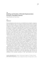
12 Chapter 2. Modeling of particulate flows
RECOVERY
COMPRESSION
CONTACT
INITIAL
Figure 2.1. Compression and recovery of two impacting particles (Zohdi [212]).

Remark. Later in the analysis, it is convenient to employ the following (per unit
mass
2
) decompositions for the key near-field parameters for the force imparted on particle
i by particle j, and vice versa:
10
• α
1ij
= α
1
m
i
m
j
,
• α
2ij
= α
2
m
i
m
j
.
2.2 Mechanical contact with near-field interaction
We now consider cases where mechanical contact occurs between particles in the presence
of near-field interaction. A primary simplifying assumption is made: the particles remain
spherical after impact, i.e., any permanent deformation is considered negligible. For two
colliding particles i and j, normal to the line of impact, a balance of linear momentum
relating the states before impact (time = t) and after impact (time = t + δt) reads as

m
i
v
in
(t) +m
j
v
jn
(t) +

t+δt
t
E
i
·n
ij
dt +

t+δt
t
E
j
·n
ij
dt = m
i
v
in
(t +δt)+m
j

v
jn
(t +δt),
(2.5)
where the subscript n denotes the normal component of the velocity (along the line con-
necting particle centers) and the E’s represent all forces induced by near-field interaction
with other particles, as well as all other external forces, if any, applied to the pair. If one
isolates one of the members of the colliding pair, then
m
i
v
in
(t) +

t+δt
t
I
n
dt +

t+δt
t
E
i
· n
ij
dt = m
i
v
in

(t +δt), (2.6)
where

t+δt
t
I
n
dt isthe totalnormal impulse dueto impact. For a pair ofparticles undergoing
impact, let usconsider a decomposition of the collision event (Figure 2.1) into a compression
(δt
1
) and a recovery (δt
2
) phase, i.e., δt = δt
1
+δt
2
. Between the compression and recovery
10
Alternatively, if the near-fields are related to the amount of surface area, this scaling could be done per unit
area.
05 book
2007/5/15
page 13
✐
✐
✐
✐
✐
✐

✐
✐
2.2. Mechanical contact with near-field interaction 13
phases, the particles achieve a common velocity,
11
denoted by v
cn
, at the intermediate time
t +δt
1
. We may write for particle i, along the normal, in the compression phase of impact,
m
i
v
in
(t) +

t+δt
1
t
I
n
dt +

t+δt
1
t
E
i
· n

ij
dt = m
i
v
cn
,
(2.7)
and, in the recovery phase,
m
i
v
cn
+

t+δt
t+δt
1
I
n
dt +

t+δt
t+δt
1
E
i
· n
ij
dt = m
i

v
in
(t +δt).
(2.8)
For the other particle (j), in the compression phase,
m
j
v
jn
(t) −

t+δt
1
t
I
n
dt +

t+δt
1
t
E
j
· n
ij
dt = m
j
v
cn
,

(2.9)
and, in the recovery phase,
m
j
v
cn
−

t+δt
t+δt
1
I
n
dt +

t+δt
t+δt
1
E
j
· n
ij
dt = m
j
v
jn
(t +δt).
(2.10)
This leads to an expression for the coefficient of restitution:
e

def
=

t+δt
t+δt
1
I
n
dt

t+δt
1
t
I
n
dt
=
m
i
(v
in
(t +δt) − v
cn
) − E
in
(t +δt
1
,t + δt)
m
i

(v
cn
− v
in
(t)) − E
in
(t, t +δt
1
)
=
−m
j
(v
jn
(t +δt) − v
cn
) + E
jn
(t +δt
1
,t + δt)
−m
j
(v
cn
− v
jn
(t)) + E
jn
(t, t +δt

1
)
,
(2.11)
where
E
in
(t +δt
1
,t + δt)
def
=

t+δt
t+δt
1
E
i
· n
ij
dt,
E
jn
(t +δt
1
,t + δt)
def
=

t+δt

t+δt
1
E
j
· n
ij
dt,
E
in
(t, t +δt
1
)
def
=

t+δt
1
t
E
i
· n
ij
dt,
E
jn
(t, t +δt
1
)
def
=


t+δt
1
t
E
j
· n
ij
dt.
(2.12)
If we eliminate v
cn
, we obtain an expression for e:
e =
v
jn
(t +δt) − v
in
(t +δt) + 
ij
(t +δt
1
,t + δt)
v
in
(t) − v
jn
(t) + 
ij
(t, t +δt

1
)
,
(2.13)
11
A common normal velocity for particles should be interpreted as indicating that the relative velocity in the
normal direction between particle centers is zero.
05 book
2007/5/15
page 14
✐
✐
✐
✐
✐
✐
✐
✐
14 Chapter 2. Modeling of particulate flows
where
12

ij
(t +δt
1
,t + δt)
def
=
1
m

i
E
in
(t +δt
1
,t + δt) −
1
m
j
E
jn
(t +δt
1
,t + δt) (2.14)
and

ij
(t, t +δt
1
)
def
=
1
m
i
E
in
(t, t +δt
1
) −

1
m
j
E
jn
(t, t +δt
1
).
(2.15)
Thus, we may rewrite Equation (2.13) as
v
jn
(t +δt) = v
in
(t +δt) − 
ij
(t +δt
1
,t + δt) + e

v
in
(t) − v
jn
(t) + 
ij
(t, t +δt
1
)


.
(2.16)
It is convenient to denote the average force acting on the particle from external sources as
E
in
def
=
1
δt

t+δt
t
E
i
· n
ij
dt. (2.17)
If e is explicitly known, then, combining Equations (2.13) and (2.5), one can write
v
in
(t +δt) =
m
i
v
in
(t) + m
j
(v
jn
(t) − e(v

in
(t) − v
jn
(t)))
m
i
+ m
j
+
(
E
in
+ E
jn
)δt −m
j
(e
ij
(t, t +δt
1
) − 
ij
(t +δt
1
,t + δt))
m
i
+ m
j
,

(2.18)
and, once v
in
(t +δt) is known, one can subsequently also solve for v
jn
(t +δt) via Equation
(2.16).
Remark. Later, it will be useful to define the average impulsive normal contact force
between the particles acting during the impact event as
I
n
def
=
1
δt

t+δt
t
I
n
dt =
m
i
(v
in
(t +δt) − v
in
(t))
δt
−

E
in
. (2.19)
In particular, as will be done later in the analysis, when we discretize the equations of
motion with a discrete (finite difference) time step of t, where δt  t, we shall define
the impulsive normal contact contribution to the total force acting on a particle, 
tot
i
=

nf
i
+ 
con
i
+ 
fric
i
(Equation (2.2)), to be

con
=
I
n
δt
t
n
ij
. (2.20)
Furthermore, at the implementation level, we choose δt = γt, where 0 <γ  1 and t

is the time step discretization size, which will be introduced later in the work.
13
We assume
δt
1
+ δt
2
= δt
1
+ eδt
1
, which immediately allows the definitions
δt
1
=
γt
1 + e
and δt
2
=
eγ t
1 + e
. (2.21)
12
This collapses to the classical expression for the ratio of the relative velocities before and after impact if the
near-field forces are negligible:
e
def
=
v

jn
(t +δt) −v
in
(t +δt)
v
in
(t) − v
jn
(t)
.
13
A typical choice is 0 <γ ≤ 0.01. Typically, the system is insensitive to γ below 0.01.
05 book
2007/5/15
page 15
✐
✐
✐
✐
✐
✐
✐
✐
2.3. Kinetic energy dissipation 15
V(0)V(0)
t
n
Figure 2.2. Two identical particles approaching one another (Zohdi [212]).
These results are consistent with the fact that the recovery time vanishes (all compression
and no recovery) for e → 0 (asymptotically “plastic”) and, as e → 1, the recovery time

equals the compression time (δt
2
= δt
1
, asymptotically “elastic”). If e = 1, there is no loss
in energy, while if e = 0, there is a maximum loss in energy. For a more detailed analysis
of impact duration times, see Johnson [111].
Remark. It is obvious that for a deeper understanding of the fields within a particle,
it must be treated as a deformable continuum. This will inevitably require the spatial
discretization, for example, using the finite element method (FEM), of the body (particle).
The implementation, theory, and application of FEM is the subject of an immense literature.
For general references on the subject, see the well-known books of Bathe [18], Becker
et al. [19], Hughes [95], Szabo and Babúska [185], and Zienkiewicz and Taylor [207].
For work specifically focusing on the continuum mechanics of particles, see Zohdi and
Wriggers [216]. For a detailed numerical analysis of multifield interaction between bodies,
see Wriggers [203].
2.3 Kinetic energy dissipation
Consider two identical particles approaching one another (Figure 2.2) in the absence of
near-field interaction. One can directly write for the kinetic energy (T ), before and after
impact,
T(t + δt) − T(t)= T (t )(e
2
− 1) ≤ 0, (2.22)
thus indicating the rather obvious fact that energy is lost with each subsequent impact for
e<1. Now consider a group of flowing particles, each with different velocity. We may
decompose the velocity of each particle by defining
v
cm
=
1

M
N
p

i=1
m
i
v
i
(2.23)
and M =

N
p
i=1
m
i
, leading to
v
i
(t) = v
cm
(t) + δv
i
(t), (2.24)
05 book
2007/5/15
page 16
✐
✐

✐
✐
✐
✐
✐
✐
16 Chapter 2. Modeling of particulate flows
where v
cm
(t) is the mean velocity of the group of particles and δv
i
(t) is a purely fluctuating
(about the mean) part of the velocity. For the entire group of particles at time = t,
N
p

i=1
m
i
v
i
(t) · v
i
(t) =
N
p

i=1
m
i

(v
cm
(t) + δv
i
(t)) · (v
cm
(t) + δv
i
(t))
= Mv
cm
(t) · v
cm
(t) + 2v
cm
(t) ·
N
p

i=1
m
i
δv
i
(t)

 
=0
+
N

p

i=1
m
i
δv
i
(t) · δv
i
(t).
(2.25)
For any later stage, the mean velocity (v
cm
) remains constant, and we have
N
p

i=1
m
i
(v
i
(t +δt) · v
i
(t +δt)) = Mv
cm
(t) · v
cm
(t) +
N

p

i=1
m
i
δv
i
(t +δt) · δv
i
(t +δt).
(2.26)
Subtracting Equation (2.25) from Equation (2.26) yields
N
p

i=1
m
i
v
i
(t +δt) · v
i
(t +δt) −
N
p

i=1
m
i
v

i
(t) · v
i
(t)
=
N
p

i=1
m
i
δv
i
(t +δt) · δv
i
(t +δt) −
N
p

i=1
m
i
δv
i
(t) · δv
i
(t)
≥ e
2
N

p

i=1
m
i
δv
i
(t) · δv
i
(t) −
N
p

i=1
m
i
δv
i
(t) · δv
i
(t)
= (e
2
− 1)
N
p

i=1
m
i

δv
i
(t) · δv
i
(t),
≥ (e
2
− 1)
N
p

i=1
m
i
v
i
(t) · v
i
(t),
(2.27)
where the first inequality arises because not all particles will experience an impact from one
stage to the next and the second inequality arises because the perturbation’s energy (that
associated with δv) must be smaller than the total (that associated with v). Thus, in the
absence of near-field interaction, we should expect
e
2
− 1 ≤
T(t + δt) − T(t)
T(t)
≤ 0. (2.28)

Remark. In order to help characterize the overall behavior of the motion, it is advan-
tageous to decompose the kinetic energy per unit mass into the bulk motion of the center of
mass and the motion relative to the center of mass:
T(t)=
T(t)
M
=
1
2
v
cm
(t) · v
cm
(t)

 
def
=T
b
= bulk motion energy
+
1
2M
N
p

i=1
m
i
δv

i
(t) · δv
i
(t)

 
def
=T
r
= relative motion energy
. (2.29)
05 book
2007/5/15
page 17
✐
✐
✐
✐
✐
✐
✐
✐
2.4. Incorporating friction 17
Clearly, theidentification of the“bulk” and “relative”parts isimportant in someapplications,
and this decomposition provides a natural way of characterizing the particulate flow.
14
We
note that the system momentum is conserved provided there are no external forces applied
to the entire system. For values of e<1, the relative motion will eventually “die out” if no
near-field forces are present.

Remark. Sometimes expressions of the form
N
p

i=1
m
i
v
i
· v
i
− Mv
cm
· v
cm
=
N
p

i=1
m
i
δv
i
· δv
i
(2.30)
are termed “granular gas temperatures.”
2.4 Incorporating friction
To incorporate frictional stick-slip phenomena during impact, for a general particle pair (i

and j ), the tangential velocities at the beginning of the impact time interval (time = t) are
computed by subtracting the relative normal velocity from the total relative velocity:
v
jt
(t) − v
it
(t) = (v
j
(t) − v
i
(t)) −

(v
j
(t) − v
i
(t)) · n
ij

n
ij
. (2.31)
One then writes the equation for tangential momentum change during impact for the ith
particle:
m
i
v
it
(t) − I
f

δt + E
it
δt = m
i
v
ct
, (2.32)
where the friction contribution is
I
f
=
1
δt

t+δt
t
I
f
dt, (2.33)
the total contribution from all other particles in the tangential direction (τ
ij
)is
E
it
=
1
δt

t+δt
t

E
i
· τ
ij
dt, (2.34)
and v
ct
is the common velocity of particles i and j in the tangential direction.
15
Similarly,
for the jth particle we have
m
j
v
jt
(t) + I
f
δt + E
jt
δt = m
j
v
ct
. (2.35)
There are two unknowns,
I
f
and v
ct
. The main quantity of interest is I

f
, which can be
solved for as
I
f
=

E
it
m
i
−
E
jt
m
j

δt + v
it
(t) − v
jt
(t)

1
m
i
+
1
m
j


δt
. (2.36)
14
An example is mixing processes.
15
They do not move relative to one another.
05 book
2007/5/15
page 18
✐
✐
✐
✐
✐
✐
✐
✐
18 Chapter 2. Modeling of particulate flows
t
n
V(0)
V(0)
Figure 2.3. Two identical particles approaching one another (Zohdi [212]).
Thus, consistent with stick-slip models of Coulomb friction, one first assumes that no slip
occurs. If
|
I
f
| >µ

s
|I
n
|, (2.37)
where
µ
s
≥ µ
d
(2.38)
is the coefficient of static friction, then slip must occur and a dynamic sliding friction model
is used. If sliding occurs, the friction force is assumed to be proportional to the normal force
and opposite to the direction of relative tangential motion, i.e.,

fric
i
def
= µ
d
||
con
||
v
jt
− v
it
||v
jt
− v
it

||
=−
fric
j
.
(2.39)
2.4.1 Limitations on friction coefficients
There are limitations on the friction coefficients for such models to make physical sense. For
example, reconsider the simple case of two identical particles (Figure 2.3), in the absence
of near-field forces, approaching one another with velocity v(t), which can be decomposed
into normal and tangential components:
v(t) = v
n
(t)e
n
+ v
τ
(t)e
τ
. (2.40)
Now consider the pre- and postimpact kinetic energy, which is identical for each of the
particles, assuming sliding (dynamic friction):
T(t)=
1
2
m(v
2
n
(t) + v
2

τ
(t))
(2.41)
and
T(t + δt) =
1
2
m(v
2
n
(t +δt) + v
2
τ
(t +δt)).
(2.42)
Assuming sliding takes place, for either particle, the impulse-momentum relation can be
written as
mv
n
(t) +

t+δt
t
I
n
dt = mv
n
(t +δt) (2.43)
05 book
2007/5/15

page 19
✐
✐
✐
✐
✐
✐
✐
✐
2.4. Incorporating friction 19
in the normal direction and
mv
t
(t) −

t+δt
t
µ
d
I
n
dt = mv
t
(t +δt) (2.44)
in the tangential direction. For the normal direction,

t+δt
t
I
n

dt = m(v
n
(t +δt) − v
n
(t)) =−(1 + e)mv
n
(t). (2.45)
Substituting this relation into the conservation of momentum relation in the tangential di-
rection, we have
v
τ
(t +δt) = v
τ
(t) − (1 + e)v
n
(t)µ
d
. (2.46)
Now consider the restriction that the friction forces cannot be so large that they reverse the
initial tangential motion. Mathematically, this restriction can be written as
v
τ
(t +δt) = v
τ
(t) − (1 + e)v
n
(t)µ
d
≥ 0, (2.47)
which leads to the expression

µ
d
≤
v
t
(t)
v
n
(t)(1 + e)
. (2.48)
Thus, the dynamic coefficient of friction must be restricted in order to make physical sense.
Qualitatively, as e grows the restrictions on the coefficients of friction are more severe,
although the author has determined that, typically, values of µ
d
≤ 0.5 are usually acceptable
for the applications considered. For more general analyses of the validity of mechanical
models involving friction, see, for example, Oden and Pires [154], Martins and Oden [147],
Kikuchi and Oden [123], Klarbring [125], Tuzun and Walton [196], or Cho and Barber [42].
Remark. One can determine the coefficient of friction that maximizes energy loss by
substituting Equation (2.46) into (2.42) and computing
∂T(t + δt)
∂µ
d
= 0 ⇒ µ
∗
d
=
v
t
(t)

v
n
(t)(1 + e)
, (2.49)
which is the maximum value of µ
d
dictated by Equation (2.48).
16
2.4.2 Velocity-dependent coefficients of restitution
It is important to realize that, in reality, the phenomenological parameter e depends on the
severity of the impact velocity. For extensive experimental data, see Goldsmith [79], or
see Johnson [111] for a more detailed analytical treatment. Qualitatively, the coefficient of
restitution has behavior as shown in Figure 2.4. A mathematical idealization of the behavior
can be constructed as
e
def
= max

e
o

1 −
v
n
v
∗

,e
−


, (2.50)
16
The second derivative indicates
∂
2
T(t+δt)
∂µ
2
d
> 0, so µ
∗
d
is a minimizer of T(t + δt). This result, which is
intuitive, implies that increasing the sliding friction coefficients allows more energy to be dissipated.