An Introduction to Modeling and Simulation of Particulate Flows Part 3 pdf

05 book
2007/5/15
page 20
✐
✐
✐
✐
✐
✐
✐
✐
20 Chapter 2. Modeling of particulate flows
IMPACT VELOCITY
e
−
EMPIRICALLY
OBSERVED
e
e
o
IDEALIZATION
V*
Figure 2.4. Qualitative behavior of the coefficient of restitution with impact ve-
locity (Zohdi [212]).
where v
∗
is a critical threshold velocity (normalization) parameter, the relative velocity of
approach is defined by
v
n
def

=|v
jn
(t) − v
in
(t)|, (2.51)
and e
−
is a lower limit to the coefficient of restitution.
05 book
2007/5/15
page 21
✐
✐
✐
✐
✐
✐
✐
✐
Chapter 3
Iterative solution schemes
3.1 Simple temporal discretization
Generally, methods for the time integration of differential equations fall within two broad
categories: (1) implicit and (2) explicit. In order to clearly distinguish between the two
approaches, we study a generic equation of the form
˙r = G(r, t). (3.1)
If we discretize the differential equation,
˙r ≈
r(t +t) −r(t)
t

≈ G(r, t). (3.2)
A primary question is, at which time should we evaluate the equation? If we use time = t,
then
˙r|
t
=
r(t +t) −r(t)
t
= G(r(t), t) ⇒ r(t +t) = r(t) + tG(r(t), t), (3.3)
which yields an explicit expression for r(t + t). This is often referred to as a forward
Euler scheme. If we use time = t + t , then
˙r|
t+t
=
r(t +t) −r(t)
t
= G(r(t + t), t + t), (3.4)
and therefore
r(t +t) = r(t) +tG(r(t + t ), t + t), (3.5)
which yields an implicit expression, which can be nonlinear in r(t +t), depending on G.
This is often referred to as a backward Euler scheme. These two techniques illustrate the
most basic time-stepping schemes used in the scientific community, which form the founda-
tion for the majority of more sophisticated methods. Two main observations can be made:
• The implicit method usually requires one to solve a (nonlinear) equation in r(t +t).
• The explicit method has the major drawback that the step size t may have to be very
small to achieve acceptable numerical results. Therefore, an explicit simulation will
usually require many more time steps than an implicit simulation.
21
05 book
2007/5/15

page 22
✐
✐
✐
✐
✐
✐
✐
✐
22 Chapter 3. Iterative solution schemes
3.2 An example of stability limitations
Generally speaking, a key difference between the explicit and implicit schemes is their
stability properties. By stability, we mean that errors made at one stage of the calculations
do not cause increasingly larger errors as the computations are continued. For illustration
purposes, consider applying each method to the linear scalar differential equation
˙r =−cr, (3.6)
where r(0) = r
o
and c is a positive constant. The exact solution is r(t) = r
o
e
−ct
. For the
explicit method,
˙r ≈
r(t +t) −r(t)
t
=−cr(t), (3.7)
which leads to the time-stepping scheme
r(Lt) = r

o
(1 − ct)
L
, (3.8)
where L indicatesthe time step counter, t = Lt for uniformtime steps (as inthis example),
and r
L
def
= r(t), etc. It is stable if |1 − ct| < 1. For the implicit method,
˙r ≈
r(t +t) −r(t)
t
=−cr(t +t), (3.9)
which leads to the time-stepping scheme
r(Lt) =
r
o
(1 + ct)
L
. (3.10)
Since
1
1+ct
< 1, it is always stable. Note that the approximation in Equation (3.8) oscillates
in an artificial, nonphysical manner when
t >
2
c
. (3.11)
If c  1, then Equation (3.6) is a so-called stiff equation, and t may have to be very small

for the explicit method to be stable, while, for this example, a larger value of t can be
used with the implicit method. This motivates the use of implicit methods, with adaptive
time stepping, which will be used throughout the remaining analysis.
3.3 Application to particulate flows
Implicit time-stepping methods, with time step size adaptivity, built on approaches found
in Zohdi [209], will be used throughout the upcoming analysis. Accordingly, after time
discretization of the acceleration term in the equations of motion for a particle (Equation
(3.1)),
¨
r
L+1
i
≈
r
L+1
i
− 2r
L
i
+ r
L−1
i
(t)
2
, (3.12)
05 book
2007/5/15
page 23
✐
✐

✐
✐
✐
✐
✐
✐
3.3. Application to particulate flows 23
one arrives at the following abstract form, for the entire system of particles:
A(r
L+1
) = F. (3.13)
It is convenient to write
A(r
L+1
) − F = G(r
L+1
) − r
L+1
+ R = 0, (3.14)
where R is a remainder term that does not depend on the solution, i.e.,
R = R(r
L+1
). (3.15)
A straightforward iterative scheme can be written as
r
L+1,K
= G(r
L+1,K−1
) + R, (3.16)
where K = 1, 2, 3, is the index of iteration within time step L +1. The convergence of

such ascheme depends onthe behavior of G. Namely, a sufficient condition for convergence
is that G be a contraction mapping for all r
L+1,K
, K = 1, 2, 3, In order to investigate
this further, we define the iteration error as

L+1,K
def
= r
L+1,K
− r
L+1
. (3.17)
A necessary restriction for convergence is iterative self-consistency, i.e., the “exact” (dis-
cretized) solution must be represented by the scheme
G(r
L+1
) + R = r
L+1
. (3.18)
Enforcing this restriction, a sufficient condition for convergence is the existence of a con-
traction mapping
||
L+1,K
||=||r
L+1,K
− r
L+1
||
=||G(r

L+1,K−1
) − G(r
L+1
)|| ≤ η
L+1,K
||r
L+1,K−1
− r
L+1
||,
(3.19)
where, if
0 ≤ η
L+1,K
< 1 (3.20)
for each iteration K, then

L+1,K
→ 0 (3.21)
for any arbitrary starting value r
L+1,K=0
,asK →∞. This type of contraction condition is
sufficient, but not necessary, for convergence. In order to control convergence, we modify
the discretization of the acceleration term:
17
¨
r
L+1
≈
˙

r
L+1
−
˙
r
L
t
≈
r
L+1
−r
L
t
−
˙
r
L
t
≈
r
L+1
− r
L
t
2
−
˙
r
L
t

. (3.22)
Inserting this into
m
¨
r = 
tot
(r) (3.23)
17
This collapses to a stencil of
¨
r
L+1
=
r
L+1
−2r
L
+r
L−1
(t)
2
when the time step size is uniform.
n05 book
2007/5/15
page 24
✐
✐
✐
✐
✐

✐
✐
✐
24 Chapter 3. Iterative solution schemes
leads to
r
L+1,K
≈
t
2
m


tot
(r
L+1,K−1
)


 
G(r
L+1,K−1
)
+

r
L
+ t
˙
r

L


 
R
, (3.24)
whose convergence is restricted by
η ∝ EIG(G) ∝
t
2
m
. (3.25)
Therefore, we see that the eigenvalues of G are (1) directly dependent on the strength of
the interaction forces, (2) inversely proportional to the mass, and (3) directly proportional
to (t )
2
(at time = t). Therefore, if convergence is slow within a time step, the time step
size, which is adjustable, can be reduced by an appropriate amount to increase the rate of
convergence. Thus, decreasing the time step size improves the convergence; however, we
want to simultaneously maximize the time step sizes to decrease overall computing time
while still meeting an error tolerance on the numerical solution’s accuracy. In order to
achieve this goal, we follow an approach found in Zohdi [208], [209], originally developed
for continuum thermochemical multifield problems in which (1) one approximates
η
L+1,K
≈ S(t)
p
(3.26)
(S is a constant) and (2) one assumes that the error within an iteration behaves according to
(S(t)

p
)
K
||
L+1,0
||=||
L+1,K
||, (3.27)
K = 1, 2, ,where ||
L+1,0
|| is the initial norm of the iterative error and S is intrinsic to
the system.
18
Our goal is to meet an error tolerance in exactly a preset number of iterations.
To this end, we write
(S(t
tol
)
p
)
K
d
||
L+1,0
|| = TOL, (3.28)
where TOL is a tolerance and K
d
is the number of desired iterations.
19
If the error tolerance

is not met in the desired number of iterations, the contraction constant η
L+1,K
is too large.
Accordingly, one can solve for a new smaller step size under the assumption that S is
constant:
t
tol
= t




TOL
||
L+1,0
||

1
pK
d

||
L+1,K
||
||
L+1,0
||

1
pK




(3.29)
The assumption that S is constant is not critical, since the time steps are to be recursively
refined and unrefined throughout the simulation. Clearly, the expression in Equation (3.29)
can also be used for time step enlargement if convergence is met in fewer than K
d
iterations.
Remark. Time step size adaptivity is important, since the flow’s dynamics can dra-
matically change over the course of time, possibly requiring quite different time step sizes to
control the iterative error. However, to maintain the accuracy of the time-stepping scheme,
one must respect an upper bound dictated by the discretization error, i.e., t ≤ t
lim
.
18
For the class of problems under consideration, due to the quadratic dependency on t, typically p ≈ 2.
19
Typically, K
d
is chosen to be between five and ten iterations.
05 book
2007/5/15
page 25
✐
✐
✐
✐
✐
✐

✐
✐
3.3. Application to particulate flows 25
Remark. Classical solution methods require O(N
3
) operations, whereas iterative
schemes, such as the one presented, typically require order N
q
, where 1 ≤ q ≤ 2. For
details, see Axelsson [11]. Also, such solvers are highly advantageous, since solutions to
previous time steps can be used as the first guess to accelerate the solution procedure.
Remark. A recursive iterative scheme of Jacobi type, where the updates are made
only after one complete system iteration, was illustrated here only for algebraic simplicity.
The Jacobi method is easier to address theoretically, while the Gauss–Seidel method, which
involves immediately using the most current values, when they become available, is usually
used at the implementation level. As is well known, under relatively general conditions, if
the Jacobi method converges, the Gauss–Seidel method converges at a faster rate, while if
the Jacobi method diverges, the Gauss–Seidel method diverges at a faster rate (for example,
see Ames [5] or Axelsson [11]). The iterative approach presented can also be considered
as a type of staggering scheme. Staggering schemes have a long history in the computa-
tional mechanics community. For example, see Park and Felippa [161], Zienkiewicz [206],
Schrefler [173], Lewis et al. [133], Doltsinis [52], [53], Piperno [162], Lewis and Schrefler
[132], Armero and Simo [7]–[9], Armero [10], Le Tallec and Mouro [131], Zohdi [208],
[209], and the extensive works of Farhat and coworkers (Piperno et al. [163], Farhat et al.
[65], Lesoinne and Farhat [130], Farhat and Lesoinne [66], Piperno and Farhat [164], and
Farhat et al. [67]).
Remark. It is important to realize that the Jacobi method is perfectly parallelizable.
In other words, the calculations for each particle are uncoupled, with the updates only
coming afterward. Gauss–Seidel, since it requires the most current updates, couples the
particle calculations immediately. However, these methods can be combined to create

hybrid approaches whereby the entire particulate flow is partitioned into groups and within
each group a Gauss–Seidel method is applied. In other words, for a group, the positions of
any particles from outside are initiallyfrozen, as far as calculations involving members ofthe
group are concerned. After each isolated group’s solution(particlepositions) has converged,
computed in parallel, then all positions are updated, i.e., the most current positions become
available to all members of the flow, and the isolated group calculations are repeated. See
Pöschel and Schwager [167] for a varietyofotherhigh-performancetechniques, in particular
fast contact searches.
Remark. We observe that for the entire ensemble of members one has
N
p

i=1
m
i
¨
r
i
=
N
p

i=1

tot
i
(r). (3.30)
We may decompose the total force due to external sources and internal interaction,

tot

i
(r) = 
EXT
i
(r) + 
INT
i
(r), (3.31)
to obtain
N
p

i=1
m
i
¨
r
i
=
N
p

i=1
(
EXT
i
(r) + 
INT
i
(r)) =

N
p

i=1

EXT
i
(r) +
N
p

i=1

INT
i
(r)

 
=0
. (3.32)
05 book
2007/5/15
page 26
✐
✐
✐
✐
✐
✐
✐

✐
26 Chapter 3. Iterative solution schemes
Thus, a consistency check can be made by tracking the condition






N
p

i=1

INT
i
(r)






= 0. (3.33)
This condition is usually satisfied, to an extremely high level of accuracy, by the previously
presented temporally adaptive scheme. However, clearly, this is only a necessary, but not
sufficient, condition for zero error.
Remark. An alternative solution scheme would be to attempt to compute the solution
by applying a gradient-based method like Newton’s method. However, for the class of
systems under consideration, there are difficulties with such an approach.

To see this, consider the residual defined by

def
= A(r) −F. (3.34)
Linearization leads to
(r
K
) = (r
K−1
) +∇
r
|
r
K−1
(r
K
− r
K−1
) + O(||r||
2
), (3.35)
and thus the Newton updating scheme can be developed by enforcing
(r
K
) ≈ 0, (3.36)
leading to
r
K
= r
K−1

− (A
TAN ,K−1
)
−1
(r
K−1
), (3.37)
where
A
TAN ,K
=
(
∇
r
A(r)
)
|
r
K
=
(
∇
r
(r)
)
|
r
K
(3.38)
is the tangent. Therefore, in the fixed-point form, one has the operator

G(r) = r − (A
TAN
)
−1
(r). (3.39)
For the problems considered, involving contact, friction, near-field forces, etc., it is unlikely
that the gradients of A remain positive definite, or even thatA is continuouslydifferentiable,
due to the impact events. Essentially, A will have nonconvex and nondifferentiable depen-
dence on the positions of the particles. Thus, a fundamental difficulty is the possibility of a
zero or nonexistent tangent (A
TAN
). Therefore, while Newton’s method usually converges
at a faster rate than a direct fixed-point iteration, quadratically as opposed to superlinearly,
its range of applicability is less robust.
3.4 Algorithmic implementation
An implementation of the procedure is given inAlgorithm 3.1. The overall goal is to deliver
solutions where the iterative error is controlled and the temporal discretization accuracy
dictates the upper limit on the time step size (t
lim
).
05 book
2007/5/15
page 27
✐
✐
✐
✐
✐
✐
✐

✐
3.4. Algorithmic implementation 27
(1) GLOBAL FIXED-POINT ITERATION (SET i = 1 AND K = 0):
(2) IF i>N
p
, THEN GO TO (4);
(3) IF i ≤ N
p
, THEN
(a) COMPUTE POSITION: r
L+1,K
i
≈
t
2
m
i


tot
i
(r
L+1,K−1
)

+ r
L
i
+ t
˙

r
L
i
;
(b) GO TO (2) AND NEXT FLOW PARTICLE (i = i + 1);
(4) ERROR MEASURE:
(a) 
K
def
=

N
p
i=1
||r
L+1,K
i
− r
L+1,K−1
i
||

N
p
i=1
||r
L+1,K
i
− r
L

i
||
(normalized);
(b) Z
K
def
=

K
TOL
r
;
(c) 
K
def
=


(
TOL

0
)
1
pK
d
(

K


0
)
1
pK


;
(5) IF TOLERANCE MET (Z
K
≤ 1) AND K<K
d
, THEN
(a) INCREMENT TIME: t = t + t;
(b) CONSTRUCT NEW TIME STEP: t = 
K
t;
(c) SELECT MINIMUM, t = min(t
lim
,t), AND GO TO (1);
(6) IF TOLERANCE NOT MET (Z
K
> 1) AND K = K
d
, THEN
(a) CONSTRUCT NEW TIME STEP: t = 
K
t;
(b) RESTART AT TIME = t AND GO TO (1).
Algorithm 3.1
Remark. At the implementation levelinAlgorithm 3.1, normalized(nondimensional)

error measures wereused. As with theunnormalized case, oneapproximates the error within
an iteration to behave according to
(S(t)
p
)
K
||r
L+1,1
− r
L+1,0
||
||r
L+1,0
− r
L
||

 

0
=
||r
L+1,K
− r
L+1,K−1
||
||r
L+1,K
− r
L

||

 

K
, (3.40)
K = 2, , where the normalized measures characterize the ratio of the iterative error
within a time step to the difference in solutions between time steps. Since both ||r
L+1,0
−
r
L
|| ≈ O(t) and ||r
L+1,K
− r
L
|| ≈ O(t) are of the same order, the use of normalized
or unnormalized measures makes little difference in rates of convergence. However, the
normalized measures are preferred since they have a clearer interpretation.
Remark. Convergence of an iterative scheme can sometimes be accelerated by relax-
ation methods. The basic idea in relaxation methods is to introduce a relaxation parameter,
05 book
2007/5/15
page 28
✐
✐
✐
✐
✐
✐

✐
✐
28 Chapter 3. Iterative solution schemes
γ , into the iterations:
r
L+1,K
= γ(G(r
L+1,K−1
) + R) + (1 − γ)r
L+1,K−1
. (3.41)
Since the scheme must reproduce the exact solution, we have
r
L+1
= γ(G(r
L+1
) + R) + (1 − γ)r
L+1
. (3.42)
Subtracting Equation (3.42) from Equation (3.41) yields
r
L+1,K
− r
L+1
= γ

G(r
L+1,K−1
) − G(r
L+1

)

+ (1 − γ)(r
L+1,K−1
− r
L+1
). (3.43)
One then forms
||r
L+1,K
− r
L+1
|| ≤ η
γ
||r
L+1,K−1
− r
L+1
||, (3.44)
where the parameter γ is chosen such that η
γ
≤ η, i.e., to induce faster convergence,
relative to a relaxation-free approach. The primary difficulty is that the selection of which
γ to induce faster convergence is unknown a priori. For even the linear theory, i.e., when
G is a linear operator, such parameters are unknown and are usually computed by empirical
trial and error procedures. See Axelsson [11] for reviews.
Remark. There are alternative ways of accelerating convergence. As we recall,
geometric convergence of the sequence a
1
,a

2
, ,a
K
, ,a implies
a − a
K+1
a − a
K
= <1, (3.45)
where  is a constant and a is the limit. Now consider the following sequence of terms:
a ≈ a
K
+ C
K
⇒ a − a
K
≈ C
K
,
⇒ a − a
K+1
≈ C
K+1
= (a − a
K
),
⇒ a − a
K+2
≈ C
K+2

= (a − a
K+1
),
(3.46)
where C is a constant. These equations can be solved simultaneously to yield
a ≈
a
K+2
a
K
− (a
K
)
2
a
K+2
+ a
K
− 2a
K+1
. (3.47)
If Equation (3.45) were true, then the value of a computed from Equation (3.47) would be
exact for all K. Only in rare cases will it be true, so we construct a new sequence, for all
K, from the old one:
a
K,1
=
a
K+2
a

K
− (a
K
)
2
a
K+2
+ a
K
− 2a
K+1
. (3.48)
We then repeat the procedure on the newly generated sequence:
a
K,2
=
a
K+2,1
a
K,1
− (a
K,1
)
2
a
K+2,1
+ a
K,1
− 2a
K+1,1

i
. (3.49)
05 book
2007/5/15
page 29
✐
✐
✐
✐
✐
✐
✐
✐
3.4. Algorithmic implementation 29
With each successive extrapolation, the new sequence becomes two members shorter than
the previous one. We repeat the procedure until the sequence is only one member long. The
final member is an approximation to the limit. It is remarked that the initial sequence does
not even have to be monotone for the process to converge to the true limit. This process
is frequently referred to as an Aitken-type extrapolation. For an in-depth analysis of this
procedure, see Aitken [4], Shanks [176], orArfken [6]. Such methods are sometimes useful
for extrapolating smooth numerical solutions to differential equations.
05 book
2007/5/15
page 30
✐
✐
✐
✐
✐
✐

✐
✐
05 book
2007/5/15
page 31
✐
✐
✐
✐
✐
✐
✐
✐
Chapter 4
Representative numerical
simulations
In order to illustrate how to simulate a particulate flow, we consider a group of N
p
randomly
positioned particles ina cubical domain withdimensions D×D×D. During the simulation,
if a particle escapes from the control volume, the position component is reversed and the
velocity component is retained (now incoming). Thus, for example, if the x
1
component
of the position vector for the ith particle exceeds the boundary of the control volume, then
r
ix
1
=−r
ix

1
is enforced. These boundary conditions are sometimes referred to as “periodic”
boundary conditions.
20
The particle size and volume fraction occupied are determined by
a particle/sample size ratio, which is defined via a “subvolume” size
21
V
def
=
D ×D × D
N
p
. (4.1)
The ratio between the particle radii (assumed the same for this example), denoted by b, and
the subvolume is
L
def
=
b
V
1
3
. (4.2)
The volume fraction occupied by the particles is
v
f
def
=
4πL

3
3
. (4.3)
Thus, the total volume occupied by the particles, denoted by , can be written as
ν = v
f
N
p
V, (4.4)
and the total mass is
M =
N
p

i=1
m
i
= ρν, (4.5)
20
There are many variants of this procedure.
21
D is normalized to unity in these simulations.
31
05 book
2007/5/15
page 32
✐
✐
✐
✐

✐
✐
✐
✐
32 Chapter 4. Representative numerical simulations
while that of an individual particle, assuming that all are the same size, is
m
i
=
ρν
N
p
= ρ
4
3
πb
3
i
. (4.6)
Remark. In the upcoming simulations, the classical random sequential addition al-
gorithm was used to place nonoverlapping particles into the computational domain (Widom
[200]). This algorithm was adequate for the volume fraction ranges of interest (under
30%), since its limit is on the order of 38%. To achieve higher volume fractions, there are
several more sophisticated algorithms, such as the classical equilibrium-based Metropolis
algorithm. For a detailed review of a variety of such methods, see Torquato [194]. For
much higher volume fractions, effectively packing (and “jamming”) particles to theoretical
limits (approximately 74%), a new class of methods has recently been developed, based
on simultaneous particle flow and growth, by Torquato and coworkers (see, for example,
Kansaal et al. [119] and Donev et al. [55]–[59]). This class of methods was not employed
in the present study due to the relatively moderate volume fraction range of interest here;

however, such methods appear to offer distinct computational advantages if extremely high
volume fractions are desired.
4.1 Simulation parameters
The relevant simulation parameters were
• number of particles = 100,
• (normalized) box dimension D = 1m,
• initial mean velocity field = (1.0, 0.1, 0.1) m/s,
• initial random perturbations around mean velocity = (±1.0, ±0.1, ±0.1) m/s,
• (normalized) length scale of the particles, L = 0.25, with corresponding volume
fraction v
f
=
4πL
3
3
= 0.0655 and radius b = 0.0539 m,
• mass density of the particles = 2000 kg/m
3
,
• simulation duration = 1s,
• initial time step size = 0.001 s,
• time step upper bound = 0.01 s,
• tolerance for the fixed-point iteration = 10
−6
.
The parameters
α
1
and α
2

, which represent the strength of the near-field interaction
forces per unit mass
2
, were varied to investigate the near-field effects on the overall partic-
ulate flow. During the simulations, we enforced the stability condition in Equation (1.37)
by setting (β
1
,β
2
) = (1, 2).
05 book
2007/5/15
page 33
✐
✐
✐
✐
✐
✐
✐
✐
4.2. Results and observations 33
X
0
0.2
0.4
0.6
0.8
1
Y

0.2
0.4
0.6
0.8
Z
0.2
0.4
0.6
0.8
Figure 4.1. A typical starting configuration for the types of particulate systems
under consideration.
0.1
0.2
0.3
0.4
0.5
0.6
0.7
0.8
0.9
0 0.1 0.2 0.3 0.4 0.5 0.6 0.7 0.8 0.9 1
ENERGY FRACTION
TIME
RELATIVE MOTION
CENTER OF MASS MOTION
0.25
0.3
0.35
0.4
0.45

0.5
0.55
0.6
0.65
0.7
0.75
0 0.1 0.2 0.3 0.4 0.5 0.6 0.7 0.8 0.9 1
ENERGY FRACTION
TIME
RELATIVE MOTION
CENTER OF MASS MOTION
0.25
0.3
0.35
0.4
0.45
0.5
0.55
0.6
0.65
0.7
0.75
0 0.1 0.2 0.3 0.4 0.5 0.6 0.7 0.8 0.9 1
ENERGY FRACTION
TIME
RELATIVE MOTION
CENTER OF MASS MOTION
0.25
0.3
0.35

0.4
0.45
0.5
0.55
0.6
0.65
0.7
0.75
0 0.1 0.2 0.3 0.4 0.5 0.6 0.7 0.8 0.9 1
ENERGY FRACTION
TIME
RELATIVE MOTION
CENTER OF MASS MOTION
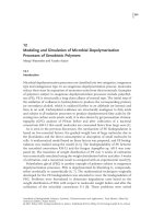
Figure 4.2. The proportions of the kinetic energy that are bulk and relative motion.
Top to bottom and left to right, for e
o
= 0.5, µ
s
= 0.2, µ
d
= 0.1: (1) no near-field
interaction, (2)
α
1
= 0.1 and α
2
= 0.05, (3) α
1
= 0.25 and α
2

= 0.125, and (4) α
1
= 0.5
and
α
2
= 0.25 (Zohdi [212]).
4.2 Results and observations
The starting configuration is shown in Figure 4.1. Figures 4.2 and 4.3 illustrate the com-
putational results. The type of motion, characterized by the proportions of bulk and rela-
05 book
2007/5/15
page 34
✐
✐
✐
✐
✐
✐
✐
✐
34 Chapter 4. Representative numerical simulations
0.51
0.52
0.53
0.54
0.55
0.56
0.57
0.58

0.59
0.6
0.61
0 0.1 0.2 0.3 0.4 0.5 0.6 0.7 0.8 0.9 1
ENERGY (N-m)
TIME
TOTAL KINETIC ENERGY
0.59
0.6
0.61
0.62
0.63
0.64
0.65
0 0.1 0.2 0.3 0.4 0.5 0.6 0.7 0.8 0.9 1
ENERGY (N-m)
TIME
TOTAL KINETIC ENERGY
0.6
0.65
0.7
0.75
0.8
0.85
0.9
0.95
0 0.1 0.2 0.3 0.4 0.5 0.6 0.7 0.8 0.9 1
ENERGY (N-m)
TIME
TOTAL KINETIC ENERGY

0.6
0.7
0.8
0.9
1
1.1
1.2
1.3
0 0.1 0.2 0.3 0.4 0.5 0.6 0.7 0.8 0.9 1
ENERGY (N-m)
TIME
TOTAL KINETIC ENERGY
Figure 4.3. The total kinetic energy in the system per unit mass. Top to bottom and
left to right, for e
o
= 0.5, µ
s
= 0.2, µ
d
= 0.1: (1) no near-field interaction, (2) α
1
= 0.1
and
α
2
= 0.05, (3) α
1
= 0.25 and α
2
= 0.125, and (4) α

1
= 0.5 and α
2
= 0.25 (Zohdi
[212]).
tive kinetic energy in the system, is dramatically different with increasing severity of the
near-field forces.
22
Notice that the kinetic energy per unit mass is nonmonotone when the
near-field interactions are taken into account (Figure 4.3). One may observe that, from
Figure 4.2, as the near-field strength is increased, the component of the kinetic energy cor-
responding to the relative motion does not decay and actually becomes dominant with time.
Essentially, the near-field interaction becomes strong enough that the flowing system expe-
riences a transition to a vibrating ensemble. This transition can be qualitatively examined
by recognizing that the governing equations are formally similar to classical, normalized,
linear (or linearized) second-order equations governing a one degree of freedom harmonic
oscillator of the form
¨r +2ζω
n
˙r +ω
2
n
r =
f(t)
m
, (4.7)
where
ω
n
=


k
m
, (4.8)
22
Typically, the simulations took under a minute on a single laptop.
05 book
2007/5/15
page 35
✐
✐
✐
✐
✐
✐
✐
✐
4.2. Results and observations 35
r is the position measured from equilibrium (r = 0), k is the stiffness associated with the
restoring force (kr), m represents the mass, and the damping ratio is
ζ
def
=
d
2mω
n
, (4.9)
d being a constant of damping and f(t) an external forcing term. The damped period of
natural, force-free vibration is
T

d
def
=
2π
ω
d
, (4.10)
where
ω
d
def
= ω
n

1 − ζ
2
(4.11)
is the “dampednatural frequency.” Using standard procedures, one decomposes thesolution
into homogeneous and particular parts:
r = r
H
+ r
P
. (4.12)
The homogeneous part must satisfy
¨r
H
+ 2ζω
n
˙r

H
+ ω
2
n
r
H
= 0. (4.13)
Assuming the standard form
r
H
= exp(λt) (4.14)
yields, upon substitution,
λ
2
exp(λt) + 2ζω
n
λ exp(λt) + ω
2
n
exp(λt) = 0, (4.15)
leading to the characteristic equation
λ
2
+ 2ζω
n
λ + ω
2
n
= 0. (4.16)
Solving for the roots yields

λ
1,2
= ω
n
(−ζ ±

ζ
2
− 1). (4.17)
The general solution is
r = A
1
exp(λ
1
t) +A
2
exp(λ
2
t). (4.18)
Depending on the value of ζ , the solution will have one of three distinct types of behavior:
• ζ>1, overdamped, leading to no oscillation, where the value of r approaches zero
for large values of time. Mathematically, λ
1
and λ
2
are negative numbers, so
r
H
= A
1

exp(ω
n
(−ζ +

ζ
2
− 1)t) + A
2
exp(ω
n
(−ζ −

ζ
2
− 1)t). (4.19)
• ζ = 1, critically damped, leading to no oscillation, where the value of r approaches
zero for largevalues of time, but faster than the overdamped solution. Mathematically,
λ
1
and λ
2
are equal real numbers, λ
1
= λ
2
=−ω
n
,so
r
H

= (A
1
+ A
2
t)exp(ω
n
t). (4.20)
05 book
2007/5/15
page 36
✐
✐
✐
✐
✐
✐
✐
✐
36 Chapter 4. Representative numerical simulations
• ζ<1, underdamped, leading to damped oscillation, where the value of r approaches
zero for large values of time, in an oscillatory fashion. Mathematically, ζ
2
− 1 < 0,
so
r
H
= A
1
cos(ω
d

t) +A
2
sin(ω
d
t). (4.21)
Thus, under certain conditions, a particulate flow can vibrate or “pulse.” The particular
solution, generated by the presence of externally applied forces, satisfies the differential
equation for a specific right-hand side:
¨r
P
+ 2ζω
n
˙r
P
+ ω
2
n
r
P
=
f(t)
m
. (4.22)
For example, if
f(t)= f
o
sin(t ), (4.23)
then
r
P

= R sin(t − φ), (4.24)
where
R =
f
o
k


1 −

2
ω
2
n

2
+

2ζ

ω
n

2
(4.25)
and
φ = tan
−1

2ζ


ω
n
1 −

2
ω
2
n

. (4.26)
Thus, clearly, such systems may resonate if forced at certain frequencies. In order to
qualitatively tie this directly to the form of problem considered in this work, consider
a linearization of a single nonlinear differential equation, describing the attraction and
repulsion from the origin (r
o
= 0) of the form
23
m¨r + d ˙r = 
nf
(r), (4.27)
where

nf
(r) =−α
1
r
−β
1
+ α

2
r
−β
2
(4.28)
and d is an effective dissipation term that would arise from inelastic impact and friction.
Upon linearization of the nonlinear interaction relation about a point r
∗
,

nf
(r) ≈ 
nf
(r
∗
) +
∂
nf
∂r




r=r
∗
(r − r
∗
) + O(r − r
∗
), (4.29)

and normalizing the equations, we obtain
¨r +2ζ
∗
ω
∗
n
˙r +(ω
∗
n
)
2
r =
f
∗
(t)
m
, (4.30)
23
The unit normal has been taken into account, thus the presence of a change in sign.
05 book
2007/5/15
page 37
✐
✐
✐
✐
✐
✐
✐
✐

4.2. Results and observations 37
where
ω
∗
n
=

−
∂
nf
∂r
|
r=r
∗
m
, (4.31)
ζ
∗
=
d
2mω
∗
n
, (4.32)
and
f
∗
(t) = 
nf
(r

∗
) −
∂
nf
∂r




r=r
∗
r
∗
. (4.33)
For the specific interaction form chosen, we have
ω
∗
n
=

−α
1
β
1
r
−β
1
−1
∗
+ α

2
β
2
r
−β
2
−1
∗
m
=

−α
1
mβ
1
r
−β
1
−1
∗
+ α
2
mβ
2
r
−β
2
−1
∗
, (4.34)

where the “loading” is
f
∗
(t) =−α
1
r
−β
1
∗
+ α
2
r
−β
2
∗
− α
1
β
1
r
−β
1
−1
∗
+ α
2
β
2
r
−β

2
−1
∗
. (4.35)
We note that if the parameters are chosen (as in the preceding simulations) specifically as
(β
1
,β
2
) = (1, 2) and r
∗
is chosen as the static equilibrium point, r
e
, given by Equation
(1.36), then
r
∗
= r
e
=
α
2
α
1
(4.36)
and
ω
∗
n
=





α
1

α
1
α
2

2
m
=

α
1
m

α
1
α
2

2
def
=

k

∗
m
, (4.37)
where
k
∗
def
= α
1

α
1
α
2

2
. (4.38)
Thus, in the preceding numerical examples, when we kept the ratio
α
1
α
2
constant, but in-
creased α
1
(while keeping m constant), we were effectively increasing the “stiffness” in the
system and, therefore, the amount of (pre)stored energy available to counteract dissipation.
Clearly, under certain conditions, a particulate flow may “pulse” (oscillate) depending on
the character of the interaction and the contact parameters. Thus, oscillatory behavior is not
unexpected for the multibody system (Figure 4.3). We remark that increasingly smaller ω

∗
n
indicates that the system tends toward a “regular” (near-field–free) particulate flow. Smaller
ω
∗
n
occurs with heavier particles or smaller attractive forces, and larger values of ζ
∗
(more
damped) occur when increased friction or smaller restitution coefficients are present in the
flow. Clearly, key dimensionless parameters, like ζ
∗
, characterize the oscillatory behavior
and the fluctuating motion with respect to mean values within the particulate flow.
05 book
2007/5/15
page 38
✐
✐
✐
✐
✐
✐
✐
✐