Analytic Number Theory A Tribute to Gauss and Dirichlet Part 9 potx
Bạn đang xem bản rút gọn của tài liệu. Xem và tải ngay bản đầy đủ của tài liệu tại đây (347.56 KB, 20 trang )
152 BEN GREEN
Definition 2.1. Fix an integer k 3. We define r
k
(N)tobethelargest
cardinality of a subset A ⊆{1, ,N} which does not contain k distinct elements
in arithmetic progression.
Erd˝os and Tur´an asked simply: what is r
k
(N)? To this day our knowledge on
this question is very unsatisfactory, and in particular we do not know the answer
to
Question 2.2. Is it true that r
k
(N) <π(N)forN>N
0
(k)?
If this is so then the primes contain k-term arithmetic progressions on density
grounds alone, irrespective of any additional structure that they might have. I do
not know of anyone who seriously doubts the truth of this conjecture, and indeed
all known lower bounds for r
k
(N) are much smaller than π(N). The most famous
such bound is Behrend’s assertion [Beh46]that
r
3
(N) Ne
−c
√
log N
;
slightly superior lower bounds are known for r
k
(N), k 4(cf.[LL, Ran61]).
The question of Erd˝os and Tur´an became, and remains, rather notorious for
its difficulty. It soon became clear that even seemingly modest bounds should
be regarded as great achievements in combinatorics. The first really substantial
advance was made by Klaus Roth, who proved
Theorem 2.3 (Roth, [Rot53]). We have r
3
(N) N (log log N)
−1
.
The key feature of this bound is that log log N tends to infinity with N,albeit
slowly
2
. This means that if one fixes some small positive real number, such as
0.0001, and then takes a set A ⊆{1, ,N} containing at least 0.0001N integers,
then provided N is sufficiently large this set A will contain three distinct elements
in arithmetic progression.
The generalisation of this statement to general k remained unproven until Sze-
mer´edi clarified the issue in 1969 for k = 4 and then in 1975 for general k.His
result is one of the most celebrated in combinatorics.
Theorem 2.4 (Szemer´edi [Sze69, Sze75]). We have r
k
(N)=o(N) for any
fixed k 3.
Szemer´edi’s theorem is one of many in this branch of combinatorics for which
the bounds, if they are ever worked out, are almost unimaginably weak. Although
it is in principle possible to obtain an explicit function ω
k
(N), tending to zero as
N →∞,forwhich
r
k
(N) ω
k
(N)N,
to my knowledge no-one has done so. Such a function would certainly be worse
than 1/ log
∗
N (the number of times one must apply the log function to N in order
to get a number less than 2), and may even be slowly-growing compared to the
inverse of the Ackermann function.
The next major advance in the subject was another proof of Szemer´edi’s the-
orem by Furstenberg [Fur77]. Furstenberg used methods of ergodic theory, and
2
cf. the well-known quotation “log log log N has been proved to tend to infinity with N, but
has never been observed to do so”.
LONG ARITHMETIC PROGRESSIONS OF PRIMES 153
his argument is relatively short and conceptual. The methods of Furstenberg have
proved very amenable to generalisation. For example in [BL96] Bergelson and
Leibman proved a version of Szemer´edi’s theorem in which arithmetic progressions
are replaced by more general configurations (x + p
1
(d), ,x+ p
k
(d)), where the
p
i
are polynomials with p
i
(Z) ⊆ Z and p
i
(0) = 0. A variety of multidimensional
versions of the theorem are also known. A significant drawback
3
of Furstenberg’s
approach is that it uses the axiom of choice, and so does not give any explicit
function ω
k
(N).
Rather recently, Gowers [Gow98, Gow01] made a major breakthrough in
giving the first “sensible” bounds for r
k
(N).
Theorem 2.5 (Gowers). Let k 3 be an integer. Then there is a constant
c
k
> 0 such that
r
k
(N) N (log log N)
−c
k
.
This is still a long way short of the conjecture that r
k
(N) <π(N)forN
sufficiently large. However, in addition to coming much closer to this bound than
any previous arguments, Gowers succeeded in introducing methods of harmonic
analysis to the problem for the first time since Roth. Since harmonic analysis (in
the form of the circle method of Hardy and Littlewood) has been the most effective
tool in tackling additive problems involving the primes, it seems fair to say that it
was the work of Gowers which first gave us hope of tackling long progressions of
primes. The ideas of Gowers will feature fairly substantially in this exposition, but
in our paper [GTc] much of what is done is more in the ergodic-theoretic spirit of
Furstenberg and of more recent authors in that area such as Host–Kra [HK05]and
Ziegler [Zie].
To conclude this discussion of Szemer´edi’s theorem we mention a variant of it
which is far more useful in practice. This applies to functions
4
f : Z/N Z → [0, 1]
rather than just to (characteristic functions of) sets. It also guarantees many arith-
metic progressions of length k. This version does, however, follow from the earlier
formulation by some fairly straightforward averaging arguments due to Varnavides
[Var59].
Proposition 2.6 (Szemer´edi’s theorem, II). Let k 3 be an integer, and let
δ ∈ (0, 1] be a real number. Then ther e is a constant c(k, δ) > 0 such that for any
function f : Z/N Z → [0, 1] with Ef = δ we have the bound
5
E
x,d∈Z/N Z
f(x)f(x + d) f(x +(k − 1)d) c(k, δ).
We do not, in [GTc], prove any new bounds for r
k
(N). Our strategy is to
prove a relative Szemer´edi theorem. To describe this we consider, for brevity of
exposition, only the case k = 4. Consider the following table.
3
A discrete analogue of Furstenberg’s argument has now been found by Tao [Taob ]. It does
give an explicit function ω
k
(N), but once again it tends to zero incredibly slowly.
4
When discussing additive problems it is often convenient to work in the context of a finite
abelian group G. For problems involving {1, ,N} there are various technical tricks which allow
one to work in Z/N
Z,forsomeN
≈ N. In this expository article we will not bother to distinguish
between {1, ,N} and Z/N Z. For examples of the technical trickery required here, see [GTc,
Definition 9.3], or the proof of Theorem 2.6 in [Gow01].
5
We use this very convenient conditional expectation notation repeatedly. E
x∈A
f(x)isde-
fined to equal |A|
−1
P
x∈A
f(x).
154 BEN GREEN
Szemer´edi Relative Szemer´edi
{1, ,N} ?
A ⊆{1, ,N}
|A| 0.0001N
P
N
=primes N
Szemer´edi’s theorem:
A contains many 4-term APs.
Green–Tao theorem:
P
N
contains many 4-term APs.
On the left-hand side of this table is Szemer´edi’s theorem for progressions of length
4, stated as the result that a set A ⊆{1, ,N} of density 0.0001 contains many
4-term APs if N is large enough. On the right is the result we wish to prove.
Only one thing is missing: we must find an object to play the rˆole of {1, ,N}.
We might try to place the primes inside some larger set P
N
in such a way that
|P
N
| 0.0001|P
N
|, and hope to prove an analogue of Szemer´edi’s theorem for P
N
.
A natural candidate for P
N
mightbethesetofalmost primes; perhaps, for
example, we could take P
N
to be the set of integers in {1, ,N} with at most
100 prime factors. This would be consistent with the intuition, coming from sieve
theory, that almost primes are much easier to deal with than primes. It is relatively
easy to show, for example, that there are long arithmetic progressions of almost
primes [Gro80].
This idea does not quite work, but a variant of it does. Instead of a set P
N
we
instead consider what we call a measure
6
ν : {1, ,N}→[0, ∞). Define the von
Mangoldt function Λby
Λ(n):=
log p if n = p
k
is prime
0otherwise.
The function Λ is a weighted version of the primes; note that the prime number
theorem is equivalent to the fact that E
1nN
Λ(n)=1+o(1). Our measure ν will
satisfy the following two properties.
(i) (ν majorises the primes) We have Λ(n) 10000ν(n) for all 1 n N.
(ii) (primes sit inside ν with positive density) We have E
1nN
ν(n)=1+
o(1).
These two properties are very easy to satisfy, for example by taking ν =Λ,or
by taking ν to be a suitably normalised version of the almost primes. Remember,
however, that we intend to prove a Szemer´edi theorem relative to ν.Inordertodo
that it is reasonable to suppose that ν will need to meet more stringent conditions.
Theconditionsweusein[GTc] are called the linear forms condition and the
correlation condition. We will not state them here in full generality, referring the
reader to [GTc, §3] for full details. We remark, however, that verifying these
conditions is of the same order of difficulty as obtaining asymptotics for, say,
nN
ν(n)ν(n +2).
6
Actually, ν is just a function but we use the term “measure” to distinguish it from other
functions appearing in our work.
LONG ARITHMETIC PROGRESSIONS OF PRIMES 155
For this reason there is no chance that we could simply take ν = Λ, since if we
could do so we would have solved the twin prime conjecture.
We call a measure ν which satisfies the linear forms and correlation conditions
pseudorandom.
To succeed with the relative Szemer´edi strategy, then, our aim is to find a
pseudorandom measure ν for which conditions (i) and (ii) and the are satisfied.
Such a function
7
comes to us, like the almost primes, from the idea of using a sieve
to bound the primes. The particular sieve we had recourse to was the Λ
2
-sieve of
Selberg. Selberg’s great idea was as follows.
Fix a parameter R,andletλ =(λ
d
)
R
d=1
be any sequence of real numbers with
λ
1
= 1. Then the function
σ
λ
(n):=(
d|n
dR
λ
d
)
2
majorises the primes greater than R. Indeed if n>Ris prime then the truncated
divisor sum over d|n, d R contains just one term corresponding to d =1.
Although this works for any sequence λ, some choices are much better than
others. If one wishes to minimise
nN
σ
λ
(n)
then, provided that R is a bit smaller than
√
N, one is faced with a minimisation
problem involving a certain quadratic form in the λ
d
s. The optimal weights λ
SEL
d
,
Selberg’s weights, have a slightly complicated form, but roughly we have
λ
SEL
d
≈ λ
GY
d
:= µ(d)
log(R/d)
log R
,
where µ(d)istheM¨obius function. These weights were considered by Goldston and
Yıldırım [GY] in some of their work on small gaps between primes (and earlier, in
other contexts, by others including Heath-Brown). It seems rather natural, then,
to define a function ν by
ν(n):=
log Nn R
1
log R
d|n
dR
λ
GY
d
2
n>R.
The weight 1/ log R is chosen for normalisation purposes; if R<N
1/2−
for some
>0thenwehaveE
1nN
ν(n)=1+o(1).
One may more-or-less read out of the work of Goldston and Yıldırım a proof
of properties (i) and (ii) above, as well as pseudorandomness, for this function ν.
7
Actually, this is a lie. There is no pseudorandom measure which majorises the primes
themselves. One must first use a device known as the W -trick to remove biases in the primes
coming from their irregular distribution in residue classes to small moduli. This is discussed in
§3.
156 BEN GREEN
One requires that R<N
c
where c is sufficiently small. These verifications use
the classical zero-free region for the ζ-function and classical techniques of contour
integration.
Goldston and Yıldırım’s work was part of their long-term programme to prove
that
(1) liminf
n→∞
p
n+1
− p
n
log n
=0,
where p
n
is the nth prime. We have recently learnt that this programme has been
successful. Indeed together with J. Pintz they have used weights coming from a
higher-dimensional sieve in order to establish (1). It is certain that without the
earlier preprints of Goldston and Yıldırım our work would have developed much
more slowly, at the very least.
Let us conclude this section by remarking that ν will not play a great rˆole in
the subsequent exposition. It plays a substantial rˆole in [GTc], but in a relatively
non-technical exposition like this it is often best to merely remark that the measure
ν and the fact that it is pseudorandom is used all the time in proofs of the various
statements that we will describe.
3. Progressions of length three and linear bias
Let G be a finite abelian group with cardinality N.Iff
1
, ,f
k
: G → C are
any functions we write
T
k
(f
1
, ,f
k
):=E
x,d∈G
f
1
(x)f
2
(x + d) f
k
(x +(k − 1)d)
for the normalised count of k-term APs involving the f
i
.Whenallthef
i
are equal
to some function f,wewrite
T
k
(f):=T
k
(f, ,f).
When f is equal to 1
A
, the characteristic function of a set A ⊆ G,wewrite
T
k
(A):=T
k
(1
A
)=T
k
(1
A
, ,1
A
).
This is simply the number of k-term arithmetic progressions in the set A, divided
by N
2
.
Let us begin with a discussion of 3-term arithmetic progressions and the trilin-
ear form T
3
.IfA ⊆ G is a set, then clearly T
3
(A) may vary between 0 (when A = ∅)
and 1 (when A = G). If, however, one places some restriction on the cardinality of
A then the following question seems natural:
Question 3.1. Let α ∈ (0, 1), and suppose that A ⊆ G is a set with cardinality
αN.WhatisT
3
(A)?
To think about this question, we consider some examples.
Example 1 (Random set). Select a set A ⊆ G by picking each element x ∈ G to
lie in A independently at random with probability α. Then with high probability
|A|≈αN. Also, if d = 0, the arithmetic progression (x, x + d, x +2d) lies in G
with probability α
3
. Thus we expect that T
3
(A) ≈ α
3
, and indeed it can be shown
using simple large deviation estimates that this is so with high probability.
LONG ARITHMETIC PROGRESSIONS OF PRIMES 157
Write E
3
(α):=α
3
for the expected normalised count of three-term progressions
in the random set of Example 1. One might refine Question 3.1 by asking:
Question 3.2. Let α ∈ (0, 1), and suppose that A ⊆ G is a set with cardinality
αN.IsT
3
(A) ≈ E
3
(α)?
It turns out that the answer to this question is “no”, as the next example
illustrates.
Example 2 (Highly structured set, I). Let G = Z/N Z, and consider the set
A = {1, ,αN}, an interval. It is not hard to check that if α<1/2then
T
3
(A) ≈
1
4
α
2
, which is much bigger than E
3
(α) for small α.
These first two examples do not rule out a positive answer to the following
question.
Question 3.3. Let α ∈ (0, 1), and suppose that A ⊆ G is a set with cardinality
αN.IsT
3
(A) E
3
(α)?
If this question did have an affirmative answer, the quest for progressions of
length three in sets would be a fairly simple one (the primes would trivially contain
many three-term progressions on density grounds alone, for example). Unfortu-
nately, there are counterexamples.
Example 3 (Highly structured set, II). Let G = Z/N Z. Then there are sets
A ⊆ G with |A| = αN ,yetwithT
3
(A) α
10000
. We omit the details of
the construction, remarking only that such sets can be constructed
8
as unions of
intervals of length
α
N in Z/N Z.
Our discussion so far seems to be rather negative, in that our only conclusion
is that none of Questions 3.1, 3.2 and 3.3 have particularly satisfactory answers.
Note, however, that the three examples we have mentioned are all consistent with
the following dichotomy.
Dichotomy 3.4 (Randomness vs Structure for 3-term APs). Suppose that
A ⊆ G has size αN.Theneither
• T
3
(A) ≈ E
3
(α) or
• A has structure.
It turns out that one may clarify, in quite a precise sense, what is meant
by structure in this context. The following proposition may be proved by fairly
straightforward harmonic analysis. We use the Fourier transform on G,whichis
defined as follows. If f : G → C is a function and γ ∈
G a character (i.e., a
homomorphism from G to C
×
), then
f
∧
(γ):=E
x∈G
f(x)γ(x).
Proposition 3.5 (Too many/few 3APs implies linear bias). Let α, η ∈ (0, 1).
Then there is c(α, η) > 0 with the following property. Suppose that A ⊆ G is a set
with |A| = αN, and that
|T
3
(A) − E
3
(α)| η.
8
Basically one considers a set S ⊆ Z
2
formed as the product of a Behrend set in {1, ,M}
and the interval {1, ,L}, for suitable M and L, and then one projects this set linearly to Z/N Z.
158 BEN GREEN
Then there is some character γ ∈
G with the property that
|(1
A
− α)
∧
(γ)| c(α, η).
Note that when G = Z/N Z every character γ has the form γ(x)=e(rx/N).
It is the occurrence of the linear function x → rx/N here which gives us the name
linear bias.
It is an instructive exercise to compare this proposition with Examples 1 and
2 above. In Example 2, consider the character γ(x)=e(x/N ). If α is reasonably
small then all the vectors e(x/N), x ∈ A, have large positive real part and so when
the sum
(1
A
− α)
∧
(γ)=E
x∈Z/N Z
1
A
(x)e(x/N)
is formed there is very little cancellation, with the result that the sum is large.
In Example 1, by contrast, there is (with high probability) considerable can-
cellation in the sum for (1
A
− α)
∧
(γ) for every character γ.
4. Linear bias and the primes
What use is Dichotomy 3.4 for thinking about the primes? One might hope to
use Proposition 3.5 in order to count 3-term APs in some set A ⊆ G by showing
that A does not have linear bias. One would then know that T
3
(A) ≈ E
3
(α), where
|A| = αN.
Let us imagine how this might work in the context of the primes. We have the
following proposition
9
, which is an analogue of Proposition 3.5. In this proposi-
tion
10
, ν : Z/N Z → [0, ∞) is the Goldston-Yıldırım measure constructed in §2.
Proposition 4.1. Let α, η ∈ (0, 2]. Then there is c(α, η) > 0 with the following
propety. Let f : Z/N Z → R be a function with Ef = α and such that 0 f(x)
10000ν(x) for all x ∈ Z/N Z, and suppose that
|T
3
(f) −E
3
(α)| η.
Then
(2) |E
x∈Z/N Z
(f(x) − α)e(rx/N)| c(α, η)
for some r ∈ Z/N Z.
This proposition may be applied with f =Λandα =1+o(1). If we could
rule out (2), then we would know that T
3
(Λ) ≈ E
3
(1) = 1, and would thus have an
asymptotic for 3-term progressions of primes.
9
There are two ways of proving this proposition. One uses classical harmonic analysis. For
pointers to such a proof, which would involve establishing an L
p
-restriction theorem for ν for
some p ∈ (2, 3), we refer the reader to [GT06]. This proof uses more facts about ν than mere
pseudorandomness. Alternatively, the result may be deduced from Proposition 3.5 by a transfer-
ence principle using the machinery of [GTc, §6–8]. For details of this approach, which is far more
amenable to generalisation, see [GTb]. Note that Proposition 4.1 does not feature in [GTc]and
is stated here for pedagogical reasons only.
10
Recall that we are being very hazy in distinguishing between {1, ,N} and Z/N Z.
LONG ARITHMETIC PROGRESSIONS OF PRIMES 159
Sadly, (2) does hold. Indeed if N is even and r = N/2 then, observing that
most primes are odd, it is easy to confirm that
E
x∈Z/N Z
(Λ(x) − 1)e(rx/N)=−1+o(1).
That is, the primes do have linear bias.
Fortunately, it is possible to modify the primes so that they have no linear bias
using a device that we refer to as the W -trick. We have remarked that most primes
are odd, and that as a result Λ − 1 has considerable linear bias. However, if one
takes the odd primes
3, 5, 7, 11, 13, 17, 19,
and then rescales by the map x → (x −1)/2, one obtains the set
1, 2, 3, 5, 6, 8, 9,
which does not have substantial (mod 2) bias (this is a consequence of the fact
that there are roughly the same number of primes congruent to 1 and 3(mod 4)).
Furthermore, if one can find an arithmetic progression of length k in this set of
rescaled primes, one can certainly find such a progression in the primes themselves.
Unfortunately this set of rescaled primes still has linear bias, because it contains
only one element ≡ 1(mod 3). However, a similar rescaling trick may be applied to
remove this bias too, and so on.
Here, then, is the W-trick. Take a slowly growing function w(N) →∞,and
set W :=
p<w(N )
p. Define the rescaled von Mangoldt function
Λby
Λ(n):=
φ(W )
W
Λ(Wn+1).
The normalisation has been chosen so that E
Λ=1+o(1).
Λ does not have sub-
stantial bias in any residue class to modulus q<w(N), and so there is at least
hope of applying a suitable analogue of Proposition 4.1 to it.
Now it is a straightforward matter to define a new pseudorandom measure ν
which majorises
Λ. Specifically, we have
(i) (ν majorises the modified primes) We have
λ(n) 10000ν(n) for all
1 n N.
(ii) (modified primes sit inside ν with positive density) We have E
1nN
ν(n)=
1+o(1).
The following modified version of Proposition 4.1 may be proved:
Proposition 4.2. Let α, η ∈ (0, 2]. Then there is c(α, η) > 0 with the following
property. Let f : Z/N Z → R be a function with Ef = α and such that 0 f(x)
10000ν(x) for all x ∈ Z/N Z, and suppose that
|T
3
(f) −E
3
(α)| η.
Then
(3) |E
x∈Z/N Z
(f(x) − α)e(rx/N)| c(α, η)
for some r ∈ Z/N Z.
160 BEN GREEN
This may be applied with f =
Λandα =1+o(1). Now, however, condition
(3) does not so obviously hold. In fact, one has the estimate
(4) sup
r∈Z/N Z
|E
x∈Z/N Z
(
Λ(x) −1)e(rx/N)| = o(1).
To prove this requires more than simply the good distribution of
Λ in residue
classes to small moduli. It is, however, a fairly standard consequence of the Hardy-
Littlewood circle method as applied to primes by Vinogradov. In fact, the whole
theme of linear bias in the context of additive questions involving primes may be
traced back to Hardy and Littlewood.
Proposition 4.2 and (4) imply that T
3
(
Λ) ≈ E
3
(1) = 1. Thus there are infinitely
many three-term progressions in the modified (W -tricked) primes, and hence also
in the primes themselves
11
.
5. Progressions of length four and quadratic bias
We return now to the discussion of §3. There we were interested in counting
3-term arithmetic progressions in a set A ⊆ G with cardinality αN. In this section
our interest will be in 4-term progressions.
Suppose then that A ⊆ G is a set, and recall that
T
4
(A):=E
x,d∈G
1
A
(x)1
A
(x + d)1
A
(x +2d)1
A
(x +3d)
is the normalised count of four-term arithmetic progressions in A.Onemay,of
course, ask the analogue of Question 3.1:
Question 5.1. Let α ∈ (0, 1), and suppose that A ⊆ G is a set with cardinality
αN.WhatisT
4
(A)?
Examples 1,2 and 3 make perfect sense here, and we see once again that there
is no immediately satisfactory answer to Question 5.1. With high probability the
random set of Example 1 has about E
4
(α):=α
4
four-term APs, but there are
structured sets with substantially more or less than this number of APs. As in §3,
these examples are consistent with a dichotomy of the following type:
Dichotomy 5.2 (Randomness vs Structure for 4-term APs). Suppose that
A ⊆ G has size αN.Theneither
• T
4
(A) ≈ E
4
(α) or
• A has structure.
Taking into account the three examples we have so far, it is quite possible that
this dichotomy takes exactly the form of that for 3-term APs. That is to say “A
has structure” could just mean that A has linear bias:
Question 5.3. Let α, η ∈ (0, 1). Suppose that A ⊆ G is a set with |A| = αN,
and that
|T
4
(A) − E
4
(α)| η.
11
In fact, this analysis does not have to be pushed much further to get a proof of Conjecture
1.2 for k = 3, that is to say an asymptotic for 3-term progressions of primes. One simply counts
progressions x, x + d, x +2d by splitting into residue classes x ≡ b(mod W ), d ≡ b
(mod W )and
using a simple variant of Proposition 4.2.
LONG ARITHMETIC PROGRESSIONS OF PRIMES 161
Must there exist some c = c(α, η) > 0 and some character γ ∈
G with the property
that
|(1
A
− α)
∧
(γ)| c(α, η)?
That the answer to this question is no, together with the nature of the coun-
terexample, is one of the key themes of our whole work. This phenomenon was
discovered, in the context of ergodic theory, by Furstenberg and Weiss [FW96]
and then again, in the discrete setting, by Gowers [Gow01].
Example 4 (Quadratically structured set). Define A ⊆ Z/N Z to be the set of
all x such that x
2
∈ [−αN/2,αN/2]. It is not hard to check using estimates for
Gauss sums that |A|≈αN, and also that
sup
r∈Z/N Z
|E
x∈Z/N Z
(1
A
(x) −α)e(rx/N)| = o(1),
that is to say A does not have linear bias. (In fact, the largest Fourier coefficient
of 1
A
− α is just N
−1/2+
.) Note, however, the relation
x
2
− 3(x + d)
2
+3(x +2d)
2
+(x +3d)
2
=0,
valid for arbitrary x, d ∈ Z/N Z. This means that if x, x + d, x +2d ∈ A then
automatically we have
(x +3d)
2
∈ [−7αN/2, 7αN/2].
It seems, then, that if we know that x, x + d and x +2d lie in A there is a very high
chance that x +3d also lies in A. This observation may be made rigorous, and it
does indeed transpire that T
4
(A) cα
3
.
How can one rescue the randomness-structure dichotomy in the light of this
example? Rather remarkably, “quadratic” examples like Example 4 are the only
obstructions to having T
4
(A) ≈ E
4
(α). There is an analogue of Proposition 3.5 in
which characters γ are replaced by “quadratic” objects
12
.
Proposition 5.4 (Too many/few 4APs implies quadratic bias). Let α, η ∈
(0, 1). Then there is c(α, η) > 0 with the following property. Suppose that A ⊆ G
is a set with |A| = αN, and that
|T
4
(A) − E
4
(α)| η.
Then there is some quadratic object q ∈Q(κ),whereκ κ
0
(α, η), with the property
that
|E
x∈G
(1
A
(x) − α)q(x)| c(α, η).
We have not, of course, said what we mean by the set of quadratic objects Q(κ).
To give the exact definition, even for G = Z/N Z, would take us some time, and
we refer to [GTa] for a full discussion. In the light of Example 4, the reader will
not be surprised to hear that quadratic exponentials such as q(x)=e(x
2
/N )are
members of Q. However, Q(κ) also contains rather more obscure objects
13
such as
q(x)=e(x
√
2{x
√
3})
12
The proof of this proposition is long and difficult and may be found in [GTa]. It is heavily
based on the arguments of Gowers [Gow98, Gow01]. This proposition has no place in [GTc],
and it is once again included for pedagogical reasons only. It played an important rˆole in the
development of our ideas.
13
We are thinking of these as defined on {1, ,N} rather than Z/N Z.
162 BEN GREEN
and
q(x)=e(x
√
2{x
√
3} + x
√
5{x
√
7} + x
√
11),
where {x} denotes fractional part. The parameter κ governs the complexity of the
expressions which are allowed: smaller values of κ correspond to more complicated
expressions. The need to involve these “generalised” quadratics in addition to
“genuine” quadratics such as e(x
2
/N ) was first appreciated by Furstenberg and
Weiss in the ergodic theory context, and the matter also arose in the work of
Gowers.
6. Quadratic bias and the primes
It is possible to prove
14
a version of Proposition 5.4 which might be applied to
primes. The analogue of Proposition 4.1 is true but not useful, for the same reason
as before: the primes exhibit significant bias in residue classes to small moduli. As
before, this bias may be removed using the W-trick.
Proposition 6.1. Let α, η ∈ (0, 2]. Then there are c(α, η) and κ
0
(α, η) > 0
with the following propety. Let f : Z/N Z → R be a function with Ef = α and such
that 0 f(x) 10000ν(x) for all x ∈ Z/N Z, and suppose that
|T
4
(f) −E
4
(α)| η.
Then we have
(5) |E
x∈Z/N Z
(f(x) − α)q(x)| c(α, η)
for some quadratic object q ∈Q(κ) with κ κ
0
(α, η).
One is interested, of course, in applying this with f =
Λ. If we could verify
that (5) does not hold, that is to say the primes do not have quadratic bias, then
it would follow that T
4
(
Λ) ≈ E
4
(1) = 1. This means that the modified (W -tricked)
primes have many 4-term progressions, and hence so do the primes themselves
15
.
One wishes to show, then, that for fixed κ one has
(6) sup
q∈Q(κ)
|E
x∈Z/N Z
(
Λ(x) − 1)q(x)| = o(1).
Such a result is certainly not a consequence of the classical Hardy-Littlewood circle
method
16
. Generalised quadratic phases such as q(x)=e(x
√
2{x
√
3}) are partic-
ularly troublesome. Although we do now have a proof of (6), it is very long and
complicated. See [GTd] for details.
In the next section we explain how our original paper [GTc] managed to avoid
the need to prove (6).
14
As with Proposition 4.1, this proposition does not appear in [GTc], though it motivated
our work and a variant of it is used in our later work [GTb]. Once again there are two proofs.
One is based on a combination of harmonic analysis and the work of Gowers, is difficult, and
requires more facts about ν than mere pseudorandomness. This was our original argument. It
is also possible to proceed by a transference principle, deducing the result from Proposition 5.4
using the machinery of [GTc, §6–8]. See [GTb] for more details.
15
in fact, just as for progressions of length 3, this allows one to obtain a proof of Conjecture
1.2 for k = 4, that is to say an asymptotic for prime progressions of length 4. See [GTb].
16
Though reasonably straightforward extensions of the circle method do permit one to handle
genuine quadratic phases such as q(x)=e(x
2
√
2).
LONG ARITHMETIC PROGRESSIONS OF PRIMES 163
7. Quotienting out the bias - the energy increment argument
Our paper [GTc] failed to rule out the possibility that
Λ − 1 correlates with
some quadratic function q ∈Q(κ). For that reason we did not obtain a proof
of Conjecture 1.2, getting instead the weaker statement of Theorem 1.3. In this
section
17
we outline the energy increment argument of [GTc], which allowed us to
deal with the possibility that
Λ −1 does correlate with a quadratic.
We begin by writing
(7)
Λ:=1+f
0
.
Proposition 6.1 tells us that T
4
(
Λ) ≈ 1, unless f
0
correlates with some quadratic
q
0
∈Q. Suppose, then, that
|E
x∈Z/N Z
f
0
(x)q
0
(x)| η.
Then we revise the decomposition (7) to
(8)
Λ:=F
1
+ f
1
,
where F
1
is a function defined using q
0
.Infact,F
1
is basically the average of
Λ
over approximate level sets of q
0
. That is, one picks an appropriate scale
18
=1/J,
and then defines
F
1
:= E(
Λ|B
0
),
where B
0
is the σ-algebra generated by the sets x : q
0
(x) ∈ [j/J,(j +1)/J).
A variant of Proposition 6.1 implies a new dichotomy: either T
4
(
Λ) ≈ T
4
(F
1
),
or else f
1
correlates with some quadratic q
1
∈Q. Suppose then that
|E
x∈Z/N Z
f
1
(x)q
1
(x)| η.
We then further revise the decomposition (8) to
Λ:=F
2
+ f
2
,
where now
F
2
:= E(
Λ|B
0
∧B
1
),
the σ-algebra being defined by the joint level sets of q
0
and q
1
.
We repeat this process. It turns out that the algorithm stops in a finite number
s of steps, bounded in terms of η. The reason for this is that each new assumption
|E
x∈Z/N Z
f
j
(x)q
j
(x)| η
17
The exposition in this section is rather looser than in other sections. To make the argument
rigorous, one must introduce various technical devices, such as the exceptional sets which feature
in [GTc, §7,8]. We are also being rather vague about the meaning of terms such as “correlate”,
and the parameter κ involved in the definition of quadratic object. Note also that the argument
of [GTc]usessoft quadratic objects rather than the genuine ones which we are discussing here
for expositional purposes. See §8 for a brief discussion of these.
18
As we remarked, the actual situation is more complicated. There is an averaging over
possible decompositions of [0, 1] into intervals of length , to ensure that the level sets look pleasant.
There is also a need to consider exceptional sets, which unfortunately makes the argument look
rather messy.
164 BEN GREEN
implies an increased lower bound for the energy of
Λrelativetotheσ-algebra
B
0
∧···∧B
j−1
,thatistosaythequantity
E
j
:= E(
Λ|B
0
∧···∧B
j−1
)
2
.
The fact that
Λ is dominated by ν does, however, provide a universal bound for
the energy, by dint of the evident inequality
E
j
10000E(ν|B
0
∧···∧B
j−1
)
2
.
The pseudorandomness of ν allows one
19
to bound the right-hand side here by O(1).
At termination, then, we have a decomposition
Λ=F
s
+ f
s
,
where
(9) sup
q∈Q
|E
x∈Z/N Z
f
s
(x)q(x)| <η,
and F
s
is defined by
(10) F
s
:= E(
Λ|B
0
∧B
1
∧···∧B
s−1
).
A variant of Proposition 6.1 implies, together with (9), that
(11) T
4
(
Λ) ≈ T
4
(F
s
).
What can be said about T
4
(F
s
)? Let us note two things about the function F
s
.
First of all the definition (10) implies that
(12) EF
s
= E
Λ=1+o(1).
Secondly, F
s
is not too large pointwise; this is again an artifact of
Λ being dominated
by ν. We have, of course,
F
s
∞
= E(
Λ|B
0
∧B
1
∧···∧B
s−1
)
∞
10000E(ν|B
0
∧B
1
∧···∧B
s−1
)
∞
.
The pseudorandomness of ν can again be used
20
to show that the right-hand side
here is 10000 + o(1); that is,
(13) F
s
∞
10000 + o(1).
The two properties (12) and (13) together mean that F
s
behaves rather like the
characteristic function of a subset of Z/N Z with density at least 1/10000. This
suggests the use of Szemer´edi’s theorem to bound T
4
(F
s
) below. The formulation
of that theorem given in Proposition 2.6 applies to exactly this situation, and it
tells us that
T
4
(F
s
) >c
for some absolute constant c>0. Together with (11) this implies a similar lower
bound for T
4
(
Λ), which means that there are infinitely many 4-term arithmetic
progressions of primes.
19
This deduction uses the machinery of the Gowers U
3
-norm, which we do not discuss in this
survey. See [GTc, §6] for a full discussion. Of specific relevance is the fact that eν
U
3
= o(1),
which is a consequence of the pseudorandomness of eν.
20
Again, the machinery of the Gowers U
3
-norm is used.
LONG ARITHMETIC PROGRESSIONS OF PRIMES 165
Let us conclude this section with an overview of what it is we have proved. The
only facts about
Λ that we used were that it is dominated pointwise by 10000ν,
and that E
Λ is not too small. The argument sketched above applies equally well
in the general context of functions with these properties, and in the context of an
arbitrary pseudorandom measure (not just the Goldston-Yıldırım measure).
Proposition 7.1 (Relative Szemer´edi Theorem). Let δ ∈ (0, 1] be a real num-
ber and let ν be a psuedorandom measure. Then there is a constant c
(4,δ) > 0
with the fol lowing property. Suppose that f : Z/N Z → R is a function such that
0 f(x) ν(x) pointwise, and for which Ef δ. Then we have the estimate
T
4
(f) c
(4,δ).
In [GTc]weprovethesame
21
theorem for progressions of any length k 3.
Proposition 7.1 captures the spirit of our argument quite well. We first deal
with arithmetic progressions in a rather general context. Only upon completion of
that study do we concern ourselves with the primes, and this is simply a matter
of constructing an appropriate pseudorandom measure. Note also that Szemer´edi’s
theorem is used as a “black box”. We do not need to understand the proof of it,
or to have good bounds for it.
Observe that one consequence of Proposition 7.1 is a Szemer´edi theorem relative
to the primes: any subset of the primes with positive relative density contains
progressions of arbitrary length. Applying this to the set of primes congruent to
1(mod 4), we see that there are arbitrarily long progressions of numbers which are
sums of two squares.
8. Soft obstructions
Readers familiar with [GTc] may have been confused by our exposition thus
far, since “quadratic objects” play essentially no rˆole in that paper. The purpose
of this brief section is to explain why this is so, and to provide a bridge between
this survey and our paper. Further details and discussion may be found in [GTc,
§6].
Let us start by recalling §3, where a set of “obstructions” to a set A ⊆ G
having roughly E
3
(α) three-term APs was obtained. This was just the collection
of characters γ ∈
G, and we used the term linear bias to describe correlation with
one of these characters.
Let f : G → C be a function with f
∞
1. Now we observe the formula
E
a,b∈G
f(x + a)f(x + b)f(x + a + b)=
γ∈
b
G
|
f(γ)|
2
f(γ)
γ(x),
which may be verified by straightforward harmonic analysis on G. Coupled with
the fact that
γ∈
b
G
|
f(γ)|
2
1,
21
Note, however, that the definition of pseudorandom measure is strongly dependent on k.
166 BEN GREEN
a consequence of Parseval’s identity, this means that the
22
“dual function”
D
2
f := E
a,b∈G
f(x + a)f(x + b)f(x + a + b)
can be approximated by the weighted sum of a few characters. Every character is
actually equal to a dual function; indeed we clearly have D
2
(γ)=γ.
We think of the dual functions D
2
(f)assoft linear obstructions.Theymay
be used in the iterative argument of §7 in place of the genuinely linear functions,
after one has established certain algebraic closure properties of these functions (see
[GTc, Proposition 6.2])
The great advantage of these soft obstructions is that it is reasonably obvious
how they should be generalised to give objects appropriate for the study of longer
arithmetic progressions. We write D
3
(f)for
E
a,b,c
f(x + a)f(x + b)f(x + c)f(x + a + b)f(x + a + c)f (x + b + c)f(x + a + b + c).
This is a kind of sum of f over parallelepipeds (minus one vertex), whereas D
2
(f)
was a sum over parallelograms (minus one vertex). This we think of as a soft
quadratic obstruction. Gone are the complications of having to deal with explicit
generalised quadratic functions which, rest assured, only become worse when one
deals with progressions of length 5 and longer.
The idea of using these soft obstructions came from the ergodic-theory work of
Host and Kra [HK05], where very similar objects are involved.
We conclude by emphasising that soft obstructions lead to relatively soft results,
such as Theorem 1.3. To get a proof of Conjecture 1.2 it will be necessary to return
to generalised quadratic functions and their higher-order analogues.
9. Acknowledgements
I would like to thank James Cranch for reading the manuscript and advice on
using Mathematica, and Terry Tao for several helpful comments.
References
[Beh46] F. A. Behrend – “On sets of integers which contain no three terms in arithmetical
progression”, Proc. Nat. Acad. Sci. U. S. A. 32 (1946), p. 331–332.
[BL96] V. Bergelson & A. Leibman – “Polynomial extensions of van der Waerden’s and
Szemer´edi’s theorems”, J. Amer. Math. Soc. 9 (1996), no. 3, p. 725–753.
[Cho44] S. Chowla – “There exists an infinity of 3—combinations of primes in A. P”, Proc.
Lahore Philos. Soc. 6 (1944), no. 2, p. 15–16.
[ET36] P. Erd
˝
os, & P. Tur
´
an – “On some sequences of integers”, J. London Math. Soc. 11
(1936), p. 261–264.
[Fur77] H. Furstenberg – “Ergodic behavior of diagonal measures and a theorem of Szemer´edi
on arithmetic progressions”, J. Analyse Math. 31 (1977), p. 204–256.
[FW96] H. Furstenberg & B. Weiss – “A mean ergodic theorem for
(1/N )
P
N
n=1
f(T
n
x)g(T
n
2
x)”, in Convergence in ergodic theory and probability
(Columbus, OH, 1993), Ohio State Univ. Math. Res. Inst. Publ., vol. 5, de Gruyter,
Berlin, 1996, p. 193–227.
22
The subscript 2 refers to the Gowers U
2
-norm, which is relevant to the study of progressions
of length 3.
LONG ARITHMETIC PROGRESSIONS OF PRIMES 167
[GH79] E. Grosswald & P. Hagis, Jr. – “Arithmetic progressions consisting only of primes”,
Math. Comp. 33 (1979), no. 148, p. 1343–1352.
[Gow98] W. T. Gowers – “A new proof of Szemer´edi’s theorem for arithmetic progressions of
length four”, Geom. Funct. Anal. 8 (1998), no. 3, p. 529–551.
[Gow01]
, “A new proof of Szemer´edi’s theorem”, GAFA 11 (2001), p. 465–588.
[Gro80] E. Grosswald – “Arithmetic progressions of arbitrary length and consisting only of
primes and almost primes”, J. Reine Angew. Math. 317 (1980), p. 200–208.
[GTa] B. J. Green & T. C. Tao – “An inverse theorem for the Gowers U
3
-norm, with appli-
cations”, to appear in Proc. Edinbrugh Math. Soc.
[GTb]
, “Linear equations in primes”, math.NT/0606088.
[GTc]
, “The primes contain arbitrarily long arithmetic progressions”, to appear in
Ann. of Math.
[GTd]
, “Quadratic uniformity of the M¨obius function”, math.NT/0606087.
[GT06]
, “Restriction theory of Selberg’s sieve, with applications”, J. Th´eorie des Nom-
bres de Bordeaux 18 (2006), p. 147–182.
[GY] D. Goldston & C. Y. Yıldırım – “Small gaps between primes, I”, math.NT/0504336.
[HB81] D. R. Heath-Brown – “Three primes and an almost-prime in arithmetic progression”,
J. London Math. Soc. (2) 23 (1981), no. 3, p. 396–414.
[HK05] B. Host & B. Kra – “Nonconventional ergodic averages and nilmanifolds”, Ann. of
Math. (2) 161 (2005), no. 1, p. 397–488.
[Kra06] B. Kra – “The Green-Tao theorem on arithmetic progressions in the primes: an ergodic
point of view”, Bull. Amer. Math. Soc. (N.S.) 43 (2006), no. 1, p. 3–23 (electronic).
[LL] I. Laba & M. Lacey – “On sets of integers not containing long arithmetic progressions”,
math.CO/0108155.
[Ran61] R. A. Rankin – “Sets of integers containing not more than a given number of terms in
arithmetical progression”, Proc.Roy.Soc.EdinburghSect.A65 (1960/1961), p. 332–
344 (1960/61).
[Rot53] K. F. Roth – “On certain sets of integers”, J. London Math. Soc. 28 (1953), p. 104–109.
[Sze69] E. Szemer
´
edi – “On sets of integers containing no four elements in arithmetic progres-
sion”, Acta Math. Acad. Sci. Hungar. 20 (1969), p. 89–104.
[Sze75]
, “On sets of integers containing no k elements in arithmetic progression”, Acta
Arith. 27 (1975), p. 199–245, Collection of articles in memory of Juri˘ı Vladimiroviˇc
Linnik.
[Taoa] T. C. Tao – “A note on Goldston-Yıldırım correlation estimates”, unpublished.
[Taob]
, “A quantitative ergodic theory proof of Szemer´edi’s theorem”, preprint.
[Tao06a]
, “Arithmetic progressions and the primes”, Collectanea Mathematica extra vol-
ume (2006), p. 37–88, Proceedings, 7th International Conference on Harmonic Analysis
and Partial Differential Equations.
[Tao06b]
, “Obstructions to uniformity, and arithmetic patterns in the primes”, Quart. J.
Pure App. Math. 2 (2006), p. 199–217, special issue in honour of John H. Coates.
[Var59] P. Varnavides – “On certain sets of positive density”, J. London Math. Soc. 34 (1959),
p. 358–360.
[vdC39] J. G. van der Corput –“
¨
Uber Summen von Primzahlen und Primzahlquadraten”,
Math. Ann. 116 (1939), p. 1–50.
[Zie] T. Ziegler – “Universal characteristic factors and Furstenberg averages”, to appear in
J. Amer. Math. Soc.
School of Mathematics, University Walk, Bristol BS8 1TW, England
E-mail address:
Clay Mathematics Proceedings
Volume 7, 2007
Heegner points and non-vanishing of Rankin/Selberg
L-functions
Philippe Michel and Akshay Venkatesh
Abstract. We discuss the nonvanishing of central values L(
1
2
,f ⊗ χ), where
f is a fixed automorphic form on GL(2) and χ varies through class group
characters of an imaginary quadratic field K = Q(
√
−D), as D varies; we
prove results of the nature that at least D
1/5000
such twists are nonvanishing.
We also discuss the related question of the rank of a fixed elliptic curve E/Q
over the Hilbert class field of Q(
√
−D), as D varies. The tools used are results
about the distribution of Heegner points, as well as subconvexity bounds for
L-functions.
1. Introduction
The problem of studying the non-vanishing of central values of automorphic L-
functions arise naturally in several contexts ranging from analytic number theory,
quantum chaos and arithmetic geometry and can be approached by a great variety
of methods (ie. via analytic, geometric spectral and ergodic techniques or even a
blend of them).
Amongst the many interesting families that may occur, arguably one of the
most attractive is the family of (the central values of) twists by class group char-
acters:Letf be a modular form on PGL(2) over Q and K a quadratic field
of discriminant D.Ifχ is a ring class character associated to K,wemayform
the L-function L(s, f ⊗ χ): the Rankin-Selberg convolution of f with the θ-series
g
χ
(z)=
{0}=a⊂O
K
χ(a)e(N(a)z). Here g
χ
is a holomorphic Hecke-eigenform of
weight 1 on Γ
0
(D) with Nebentypus χ
K
and a cusp form iff χ is not a quadratic
character
1
.
2000 Mathematics Subject Classification. Primary 11F66, Secondary 11F67, 11M41.
Key words and phrases. Automorphic L-functions, Central Values, Subconvexity,
Equidistribution.
The research of the first author is partially supported by the RMT-network “Arithmetic
Algebraic Geometry” and by the “RAP” network of the R´egion Languedoc-Roussillon.
The second author was supported by the Clay Mathematics Institute and also acknowledges
support through NSF grants 02045606 and NSF Grants DMS0111298. He thanks the Institute of
Advanced Study for providing excellent working conditions.
1
Equivalently, one can define L(s, f ⊗ χ)asL(s, Π
f
⊗ χ), where Π
f
is the base-change to K
of the automorphic representation underlying f,andχ is regarded as a character of A
×
K
/K
×
.
c
2007 Philippe Michel and Akshay Venkatesh
169
170 PHILIPPE MICHEL AND AKSHAY VENKATESH
We will always assume that the conductor of f is coprime to the discriminant of
K. In that case the sign of the functional equation equals ±
−D
N
, where one takes
the + sign in the case when f is Maass, and the − sign if f is weight 2 holomorphic
(these are the only cases that we shall consider).
Many lovely results have been proved in this context: we refer the reader to
§1.3 for a review of some of these results. A common theme is the use, implicit or
explicit, of the equidistribution properties of special points. The purpose of this
paper is to give an informal exposition (see §1.1) as well as some new applications
of this idea. Since our goal is merely to illustrate what can be obtained along these
lines we have not tried to reach the most general results that can be obtained and,
in particular, we limit ourselves to the non-vanishing problem for the family of
unramified ring class characters of an imaginary quadratic field K = Q(
√
−D)of
large discriminant D.
We prove
Theorem 1. Let f(z) be a weight 0, even, Maass (Hecke-eigen) cuspform on
the modular surface X
0
(1); then, for any 0 <δ<1/2700, one has the lower bound
{χ ∈
Cl
K
,L(f ⊗χ, 1/2) =0}
δ,f
D
δ
Theorem 2. Let q be a prime and f(z) be a holomorphic Hecke-eigen cuspform
of weight 2 on Γ
0
(q) such that q remains inert in K;then,forany0 <δ<1/2700,
one has the lower bound
{χ ∈
Cl
K
,L(f ⊗χ, 1/2) =0}
δ,f
D
δ
for any δ<1/2700.
The restriction to either trivial or prime level in the theorems above is merely
for simplification (to avoid the occurrence of oldforms in our analysis) and extending
these results to more general levels is just a technical matter. Another arguably
more interesting generalization consists in considering levels q and quadratic fields
K such that the sign of the functional equation is −1: then one expects that the
number of χ such that the first derivative L
(f ⊗ χ, 1/2) =0is D
δ
for some
positive absolute δ. This can be proven along the above lines at least when f is
holomorphic of weight 2 by using the Gross/Zagier formulas; the proof however
is significantly more difficult and will be dealt with elsewhere; interestingly the
proof combines the two types of equidistribution results encountered in the proof
of Theorems 1 and 2 above. In the present paper, we give, for the sake of diversity,
an entirely different, purely geometric, argument of such a generalization when f
corresponds to an elliptic curve. For technical reasons we need to assume a certain
hypothesis “S
β,θ
” that guarantees there are enough small split primes in K.This
is a fairly common feature of such problems (cf. [DFI95], [EY03]) and we regard
it as almost orthogonal to the main issues we are considering. Given θ>0and
α ∈]0, 1] we consider
Hypothesis S
β,θ
. The number of primitive
2
integral ideals n in O
K
with
Norm(n) D
θ
is D
βθ
.
Actually, in a sense it is remarkable that Theorems 1 and 2 above do not require
such a hypothesis. It should be noted that S
β,θ
is always true under the generalized
2
That is, not divisible by any nontrivial ideal of the form (m), with m ∈ Z.
HEEGNER POINTS AND NON-VANISHING 171
Lindel¨of hypothesis and can be established unconditionally with any α ∈]0, 1/3[ for
those Ds whose largest prime factor is a sufficiently small power of D by the work
of Graham/Ringrose [GR90]( see [DFI95] for more details).
Theorem 3. Assume S
β,θ
.LetE be an elliptic curve over Q of squarefree
conductor N , and suppose D is odd, coprime to N, and so that all primes dividing
N split in the quadratic extension Q(
√
−D). Then the Mordell-Weil rank of E over
the Hilbert class field of Q(
√
−D) is
D
δ−
,whereδ =min(βθ, 1/2 −4θ).
Neither the statement nor the proof of Theorem 3 make any use of automorphic
forms; but (in view of the Gross/Zagier formula) the proof actually demonstrates
that the number of nonvanishing central derivatives L
(f
E
⊗χ, 1/2) is D
α
,where
f
E
is the newform associated to E. Moreover, we use the ideas of the proof to give
another proof (conditional on S
β,θ
)ofThm.1.
We conclude the introduction by describing the main geometric issues that
intervene in the proof of these Theorems. Let us consider just Theorem 1 for
clarity. In that case, one has a collection of Heegner points in SL
2
(Z)\H with
discriminant −D, parameterized by Cl
K
. The collection of values L(
1
2
,f ⊗ χ)
reflects – for a fixed Maass form f ,varyingχ through
Cl
K
– the distribution of
Heegner points. More precisely, it reflects the way in which the distribution of
these Heegner points interacts with the subgroup structure of Cl
K
. For example, if
there existed a subgroup H ⊂ Cl
K
such that points in the same H-coset also tend
to cluster together on SL
2
(Z)\H, this would cause the L-values to be distributed
unusually. Thus, in a sense, whatever results we are able to prove about these values
are (geometrically speaking) assertions that the group structure on Cl
K
does not
interact at all with the “proximity structure” that arises from its embedding into
SL
2
(Z)\H.
Remark 1.1. Denote by Cl
K
=Pic(O
K
) the class group of O
K
and by
Cl
K
its
dual group. We write h
K
= |Cl
K
| = |
Cl
K
| for the class number of O
K
. By Siegel’s
theorem one has
(1) h
K
ε
D
1/2−ε
(where the constant implied is not effective) so the lower bounds of Theorems 1
and 2 are far from giving a constant proportion of nonvanishing values. (In the
case where f is Eisenstein, Blomer has obtained much better results: see Sec. 1.3).
Moreover, both proofs make use of (1) so the constants implied are ineffective.
1.1. Nonvanishing of a single twist. Let us introduce some of the main
ideas of the present paper in the most direct way, by sketching two very short proofs
that at least one twist is nonvanishing in the context of Theorem 1. We denote by
H the upper-half plane. To the quadratic field K = Q(
√
−D)–wherewealways
assume that −D is a fundamental discriminant – and each ideal class x of the
maximal order O
K
of Q(
√
−D) there is associated a Heegner point [x] ∈ SL
2
(Z)\H.
3
One can describe the collection He
K
:= {[x]:x ∈ Cl
K
} using the moduli
description of SL
2
(Z)\H: if one identifies z ∈ SL
2
(Z)\H with the isomorphism
3
Namely, [x] is represented by the point
−b+
√
−D
2a
,whereau
2
+ buv + cv
2
is a quadratic form
of discriminant −D corresponding to the ideal class x, i.e. there exists a fractional ideal J in the
class x and a Z-basis α, β for J so that Norm(uα + vβ)=Norm(J)(au
2
+ buv + cv
2
).