Atomic Force Microscopy in Cell Biology Episode 2 Part 4 docx

266 Schneider et al.
hundred pN, a change that alters the indentation significantly (Fig. 6). Another
consideration is that changes in cell elasticity may occur that will change the
indentation significantly (Fig. 7). For example, the stimulation of endothelial
cells with thrombin (a mediator of inflammation that increases the permeabil-
ity of the endothelial monolayer) changes the cell elasticity by a factor of 5
(unpublished data by R. Matzke). A third point is that it is desirable to obtain
quantitative volume data. A method to circumvent the above mentioned prob-
lems is to operate the AFM in the force-mapping mode (also called force-vol-
ume mode; ref. 31). This method allows a quantification of the unindented cell
volume, independent of the loading force and independent of the elastic modu-
lus of the cell. It allows a measurement and quantification of the local cell
elasticity. The BioScope can be operated in the force volume mode. Therefore,
it would be possible to calculate actual cell height and cell volume irrespective
of cell stiffness. The BioScope software permits a qualitative analysis of the
elastic properties of the sample, but features to calculate the unindented height
and to quantify the elastic modulus are missing. In other words, it is possible to
record all the data necessary for a actual cell volume measurement, but we
cannot analyze the data with the current BioScope software. A group of
researchers, M. Radmacher, C. Rotsch and R. Matzke (Departments of Phys-
ics; Universities of Munich and Göttingen, Germany) wrote a program in IGOR
Fig. 7. Indentation of a soft sample at a constant loading force of 0.5 nN as a func-
tion of the elastic modulus of the sample. The Hertz model for a conical indenter with
a half opening angle of 35° was used for this calculation.
Aldosterone-Sensitive Cells Imaged With AFM 267
PRO (Wavemetrics, Lake Oswego, OR) to analyze the force volume data.
Please, check the Appendix and the literature (30–36) for further information.
3.9. Appendix
Force Mapping (31) allows a quantification of the unindented cell volume,
independent of the loading force and independent of the elastic modulus of the
cell. The following section explains the analysis of the data and gives practical

hints for data acquisition.
3.9.1 Force Mapping
A force map is a 2D array of force curves. (You already know a single force
curve from the force calibration menu of the BioScope.) In a force curve, the
force acting on the AFM tip is measured as the tip approaches and retracts from
the surface of a sample (Fig. 8). Typically, the cantilever starts the approach
from a point where it is not in contact with the surface. After contact, it can be
further approached until a maximal loading force is reached. Then the cantile-
ver is retracted from the surface until the tip is free again. The deflection and
the vertical position of the z piezo are recorded in such a force curve. Accord-
ing to Hooke’s law, the loading force, F, can be calculated by multiplying the
measured deflection, d, with the spring constant, k
C
, of the cantilever.
F = k
C
× d (1)
A force curve consists of two parts: the noncontact part and the contact part.
When the tip is not in contact with the surface, the deflection will be constant.
A further motion down after contact will deflect the cantilever. On a stiff
sample, this deflection is equal to the travel of the z piezo after the contact
point because the stiff sample cannot be indented (Fig. 8). However, a soft
sample will be indented by the tip. Thus, the force curve will be shallower than
on a stiff sample (Fig. 9). The indentation, δ, at a certain loading force can be
calculated as the travel of the z piezo, z, after the contact point minus the
deflection of the cantilever.
δ = z – d (2)
The unindented height of the sample can be calculated by finding the con-
tact point. The contact point can be found rather easily in the case of a stiff
sample since the force curve shows a sharp bend there (Figs. 8 and 9). In the

case of a soft sample, the exact position of the contact point is often hard to
determine since the transition between noncontact part and contact part is
very shallow (Fig. 9). The contact point may also be hidden by thermal noise.
A method to determine the contact point on a soft sample is described below.
From the contact part of a force curve the elastic modulus can be calculated
268 Schneider et al.
by analyzing the force dependent indentation. This analysis will also be
described below.
By recording a 2D array of force curves on a cell, a map of the unindented
height and a map of the local elastic properties can be calculated (Fig. 10).
3.9.2. Calculation of the Contact Point and of the Elastic Modulus
The contact part of a force curve on a soft sample is nonlinear because the
compliance of the sample becomes higher for larger loading forces. This is
attributable to a geometrical effect. AFM tips are approximately conical and
therefore the contact area increases with the increasing indentation. This pro-
cess was treated analytically first by Hertz (37) and a more general solution
was obtained by Sneddon (38). For the geometry of a conical tip indenting a
flat sample (which is most appropriate here) the relation between the indenta-
tion, δ, and the loading force, F, is given by the following:
F = δ
2
× (2/π) × [E/(1–ν
2
)] × tan(α) (3)
where ν is the Poisson ratio, E is the elastic modulus, and α is the half opening
angle of the conical tip. For incompressible materials (as assumed for cells),
the Poisson ratio is 0.5. The half opening angle for Microlever (Park Scien-
Fig. 8. Force curve on a stiff sample. Only the approach part is shown. The force
curve consists of two parts: the noncontact part and the contact part. As long as the tip
is not in contact with the surface, the deflection (and therefore the loading force) is

constant. The tip contacts the surface in the contact point. In the contact part, a further
approach deflects the cantilever. Because the stiff sample cannot be indented by the
tip, the deflection equals the travel of the z piezo after the contact point.
Aldosterone-Sensitive Cells Imaged With AFM 269
tific) is 35°. The loading force can be calculated by Eq. 1 and the indentation
can be calculated by Eq. 2. This gives the following:
k
c
× d = (z – d)
2
× (2/π) × [E/(1 – ν
2
)] × tan(α) (4)
Thus, the elastic modulus can be calculated by the measured deflection and
z-piezo position. However, in measured data the deflection of the noncontact
part of the force curve is not necessarily zero (Fig. 11). Therefore, the deflec-
tion, d, must be replaced by the following:
d → d
i
– d
0
(5)
where d
0
is the deflection offset and d
i
is a measured deflection value.
Eq. 3 is only valid for the contact part of the force curve. Thus, the contact
point z
0

must be subtracted from a measured z-piezo value, z
i
. Because the
BioScope
®
stores force curves inverted (i.e., the point with the maximal
deflection has the z-value 0 and the starting point of the approach has the maxi-
mum z value, Fig. 11), z must be replaced by the following:
Fig. 9. Force curves on a soft and on a stiff sample. Only the approach parts are
shown. The curve on the soft sample is shallower because sample is indented by the
tip. The indentation is the travel of the z piezo after the contact point minus the deflec-
tion. The curve is nonlinear because the compliance becomes higher for larger loading
forces. This is the result of a geometrical effect: AFM tips are (approximately) conical
and therefore the contact area increases with the indentation. The contact point can
very easily be determined on the stiff sample since the force curve shows a sharp bend
there. On the soft sample, the determination of the contact point is more difficult since
the transition between noncontact part and contact part is very shallow. See text for
how to find the contact point on a soft sample.
270 Schneider et al.
270
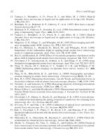
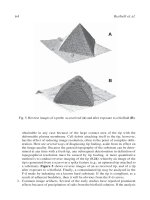
Fig. 10. Force maps of a living endothelial cell (HUVEC). (A) unindented height, (B) elastic modulus, and (C) contact mode
image of the same cell. The unindented height image (A) shows a smooth cell surface, whereas the contact mode image shows
height fluctuations (C). This is because the indentation depends on the local elastic properties; soft regions will be more indented
than stiffer regions. The cytoskeleton is a structured polymeric network with very different local elastic properties, as shown
in the
elasticity map (B). The elastic indentation leads to an underestimation of the cell volume.
Aldosterone-Sensitive Cells Imaged With AFM 271
z → z
o
– z

i
(6)
where z
0
is the z-piezo value of the contact point and z
i
is a measured z-piezo
position value (Fig. 11).
Eqs. 5 and 6 inserted in Eq. 4 gives the following:
k
c
× (d
i
– d
0
) = [(z
0
– z
i
) – (d
i
– d
0
)]
2
× (2/π) × [E/(1 – ν
2
)] × tan(α) (7)
In this equation, we have three unknown parameters: the deflection offset,
d

0
, the contact point, z
0
, and the elastic modulus, E. The deflection offset can
easily be determined by the noncontact part of the force curve. As mentioned
above, the transition from noncontact to contact part is very shallow and there-
fore the contact point cannot be determined by easy means. Unfortunately,
Eq. 7 is of such a form that an analytical least squares fit to determine E and z
0
cannot be performed. One possibility is to perform a Monte-Carlo fit with
reasonable starting values. However, the two missing parameters can be
obtained more easily. Since the signal-to-noise ratio of measured data is very
good (because thermal noise is reduced when the tip contacts the cell), we can
Fig.11. Parameters used for the calculation of the contact point and the elastic modu-
lus. The two deflection values d
1
and d
2
and their corresponding z-piezo positions z
1
and z
2
define the range of analysis. The deflection-offset d
0
is given by the noncontact
part of the force curve. With these values and Eqs. 9 and 10, the contact point z
0
and
the elastic modulus can be calculated. In this example, d
0

= 10 nm, d
1
= 40 nm, d
2
= 80
nm, z
1
= 0.5 µm, z
2
= 0.2 µm, and z
0
= 1 µm.
272 Schneider et al.
take two measured deflection values, d
1
and d
2
, and their corresponding
z-piezo values, z
1
and z
2
, of the contact part of the force curve and insert them
in Eq. 7. This gives two equations with two missing parameters, E and z
0
:
k
c
× (d
1

– d
0
) = [(z
0
– z
1
) – (d
1
– d
0
)]
2
× (2/π) × [E/(1 – ν
2
)] × tan(α) (8a)
k
c
× (d
2
– d
0
) = [(z
0
– z
2
) – (d
2
– d
0
)]

2
× (2/π) × [E/(1 – ν
2
)] × tan(α) (8b)
The contact point can be calculated by solving Eq. 8a for E and inserting E
in Eq. 8b:
z
0
=
z
2
+ d
2
d
1
– z
1
+ d
1
d
2
d
1
– d
2
(9)
The elastic modulus can now be calculated by inserting z
0
in Eq. 8a or 8b.
A better method to calculate the elastic modulus is to apply an analytical

least squares fit (this is possible now because z
0
is known) to all the data points
(d
i
/z
i
) in the range of analysis (Fig. 11) that is limited by (d
1
/z
1
) and (d
2
/z
2
):
E =
Σ
i
F
i
δ
i
2
Σ
i
δ
i
4
×

π ·1–v
2
2·tan α
(10)
where δ
i
= (z
0
– z
i
) – (d
i
– d
0
).
The BioScope stores force curves in the force volume mode in a relative
manner. This means that the absolute position of the z piezo is not recorded in
the force curve itself and every force curve starts with z = 0. The force volume
data consists of two separate datasets, one that contains the array of force
curves, and another, in which the absolute height information is stored. Each
pixel of the height image represents the absolute z-piezo value when the corre-
sponding force curve switches from approach to retract (i.e., the point with the
maximal loading force). Therefore, to calculate the unindented height, H
0
, we
have to add the calculated contact point, z
0
, to the height at maximal loading
force, H:
H

0
= H + z
0
(11)
3.9.3. How to Access the Force Volume Data from the BioScope File
A force volume measurement consists typically of 64 × 64 force curves.
Because of the amount of data, it is convenient to write a computer algorithm
to analyze the data. Unfortunately, the BioScope software cannot export force
volume data in a standard data format like ASCII. However, there is data analy-
sis software (like IGOR PRO) that can read the binary information of the
BioScope data file. At this time, it is difficult to give general advice on how to
reconstruct the data from the binary file since the file format has changed in the
past rather frequently for the various BioScope software versions. Please refer
Aldosterone-Sensitive Cells Imaged With AFM 273
to the manual of your software version to get information about the file and
data structure.
When you are measuring living cells, the AFM is operated in liquid. In this
case, the approach and retract part of the force curves are separated from each
other (Fig. 12). This separation is caused by hydrodynamic forces as the canti-
lever is dragged through the fluid medium (34). This causes a force offset that
depends on the speed of the z piezo, and the sign of that offset changes when
the direction of movement is reversed between approach and retract. One way
of dealing with this force offset is to average point by point the approach and
retract part of the force curve and use this average for further analysis.
3.9.3.1 NOTES
The Hertz model applied in the analysis is valid on condition that the sample
is thick compared with the indentation, is homogeneous, and is flat, and that
the geometry of the tip is a cone. The real situation fits these requirements only
partly. The typical height of cells in the region of the nucleus is 4 µm. Here the
height is sufficiently large versus the indentation (approx 400 nm). In the region

of the thin lamellipodium, this condition is not fulfilled. With increasing
indentation, the tip will feel the underlying stiff substrate and the force curve
Fig. 12. Force curve on a living cell in liquid medium. The approach and retract
parts are separated by hydrodynamic drag that adds a constant external force to the
loading force of the cantilever. This force-offset is speed dependent (the faster the
scan speed the bigger the force-offset; data not shown here) and changes its sign when
the direction of movement is reversed from approach to retract. One way to deal with
this force-offset is to average the approach and retract part point by point and to ana-
lyze the resulting average force curve.
274 Schneider et al.
will be initially the shape of a curve for a soft sample, but it will become
linear and appear like a curve for a stiff substrate at higher deflection values
(36). For the analysis of force curves taken on thin cell regions, it is therefore
necessary to choose a fit range with sufficiently small deflection values (32).
At small indentation values, the geometry of the AFM tip on nano-meter scale
will become important. AFM tips look like a pyramid whose top is formed by
a half sphere. The radius of that sphere is typically in the range of 50 nm. The
Hertz model for the cone is no longer appropriate here. A better description of
the data is the Hertz model for a sphere indenting a flat surface:
F =
4
3
×
E
1–v
2
×δ
3/2
× R
(12)

where R is the radius of the tip (35).
Because the area of the cell surface is large, compared to the radius of the
tip, one can assume as an approximation that the sample is flat, and thereby
satisfy the Hertz model.
Cell material is not at all homogeneous. The cytoskeleton is a polymeric
network that consists of polymers with very different elastic properties. There
might also be contributions to the measured elastic modulus from the lipid
membrane or from tension in the cytoskeleton. However, the scope of this
article is the determination of the cell volume and not the quantification of
the elastic modulus. Inhomogenieties may lead to an apparent elastic modu-
lus, i.e., an average of all elastic components that contribute to the measured
value. In practice, the contact point can be determined with sufficient preci-
sion despite this problem. If the elastic modulus changes with the depth of
indentation (as with thin lamellipodia where the tip “feels” the underlying
stiff substrate or when the elastic properties vary with the depth of indenta-
tion), one should take care that the data are analyzed in a fit range with small
deflection values. Jan Domke (unpublished observation) showed by calculat-
ing simulations that the analysis of the cell height with the Hertz model gives
reasonable values. There is only a systematic underestimation in the order of
the tip radius.
3.9.4. How to Record a Force Map
Typical settings are trigger mode: relative; trigger threshold: 100 nm; z-scan size:
1.5 µm; z-scan speed: 10 Hz; 64 points per force curve, 64 × 64 points per image.
3.9.4.1 COMMENTS
“Trigger mode: relative” means that the tip is approached to the sample until
the cantilever reaches a deflection of “trigger threshold” (in our example 100
nm), relative to the deflection offset of the force curve given by the noncontact
Aldosterone-Sensitive Cells Imaged With AFM 275
part of the curve. This ensures that the deflection (and therefore the loading
force) does not exceed the value given by trigger threshold. This prevents cell

damage caused by high loading forces and ensures that the contact part of the
scan will be long enough to find good deflection values for the data analysis.
You can compare the relative trigger threshold with the set point in the contact
mode, where the loading force can be adjusted by the set point. For the deter-
mination of the deflection offset, the force curve must contain a clear
noncontact part (typically one-fourth of the total length of the force curve). In
the BioScope, the tip is being approached until the deflection equals the trigger
threshold. Then the z piezo moves upward the length given by the z-scan size.
To get a distinct noncontact part, the z-scan size must be long enough for the
tip to become free. A good starting value is 1.5 µm on living cells. With high
cells, it might be difficult (or even impossible) to measure the topmost region
of the cell since the necessary piezo travel range of the BioScope (6 µm) might
be smaller than the height of the cell plus the z-scan range. New BioScope
versions offer piezos with extended range. The z-scan speed is limited since
hydrodynamic drag will cause a speed-dependent force offset. On the other
hand, slow scan speed increases the time necessary to record a complete force
map. A good compromise is a scan speed of 10 Hz. It will then take about 13 min
to record a force map with 64 × 64 pixels. The number of pixels determines the
lateral resolution. Of course, a small number will speed up data acquisition but
decrease lateral resolution. However, you should consider the motion of the tip
in the force-mapping mode: after recording one force curve, the tip moves lat-
erally to record the next force curve. The lateral step size is given by the total
lateral scan size divided by the number of pixels. With large step sizes, it might
happen that the tip or cantilever bumps against the cell when it moves to the
side because the tip is not far enough above the cell than the height of the cell
increases. If possible, you can either increase the z-scan size or increase the
number of pixels. Note that the BioScope cannot store more than 64 × 64 × 64
data points (64 lines × 64 columns × 64 points in the force curve). When you
increase the length of the force curve, the force resolution of the curve will
become worse. Smaller lateral pixel numbers permit more points in the force

curve (for example, 16 × 16 × 512).
4. Notes
1. How to increase your time resolution: If it is not necessary to record all three
dimensions (x-, y-, and z-axis) of the cell you can increase time resolution (up to
100 ms/line) by imaging only two dimensions (x- and z-axis). Switch the mode
from slow axis enable to slow axis disable (= line scan) in your software menu.
The cantilever is now moving back and forth along the same scanning line
(x-axis). The y-axis will not be recorded. Fast volume fluctuations upon cell
stimulation are now visible as a height increase or decrease.
276 Schneider et al.
2. Before starting cell imaging, make sure that your system provides good and stable
images on a clean glass cover slip under fluid. This will help you to distinguish
between problems that arise from the microscope (AFM tip damaged, air bubbles
stuck to the cantilever, mechanical vibrations) or problems caused by the cells
(membrane blebbing, cell detachment, etc.).
3. ECs that are under scanning should not change their morphology. You can
observe the cells constantly through the light microscope.
4. The temperature of the environment (in the box) should be close to 37°C (in
practice: approx 30°C) to minimize temperature alterations. Any increase or
decrease of the temperature in the bath solution (which must have 37°C) is fol-
lowed by artificial cantilever deflections.
5. Avoid acoustical or mechanical noise (speaking or walking) during the experiment.
6. If you cannot get an image or if you cannot increase the integral gain above 1 and
the proportional gain above 2, check or modify the following parameters:
a. Increase the loading force.
b. The glass cover slip is too thin (<0.8 mm);
c. There is a lot of noise or vibrations in your laboratory. Switch off: heating
chamber, microscopy lamps, perfusion system, etc. Install the BioScope com-
puter some distance away from the scanner and make sure that its fan does not
blow in the direction of the scanner;

d. The temperature of the bath solution is not constant;
e. There are air bubbles stuck to the cantilever;
f. The AFM tip is dirty;
g. The cells detach from the glass surface (e.g., temperature above 37°C);
h. The cells show membrane blebbing (a hint that the cells are in a bad condition
and/or get damaged by the scanning tip);
i. The glass cover slip (with the cell layer) is not firmly fixed in the perfusion
chamber and thus comes off;
j. Cell height is beyond the z piezo range of the instrument. Decrease the scan
size or try to image a flat cell surface area (i.e. lamellipodium or cell–cell
contact area). Adjust the piezo height with the step motor.
Acknowledgments
This work was supported by the VW-Stiftung (AZ I/77299) and the
Interdisziplinäre Zentrum für Klinische Forschung (IZKF, TP I/90).
References
1. Harvey, B. J. , Condliffe, S., and Doolan, C. M. (2001) Sex and salt hormones:
rapid effects in epithelia. News Physiol. Sci. 16, 174–177.
2. Wehling, M., Käsmayr, J., and Theisen, K. (1991) Rapid effects of mineralocorti-
coids on sodium exchanger: Genomic or nongenomic pathways? Am. J. Physiol.
260, E719–E726.
3. Wehling, M., Ulsenheimer, A., Schneider, M., Neylon, C., and Christ, M. (1994)
Rapid effects of aldosterone on free intracellular calcium in vascular smooth
Aldosterone-Sensitive Cells Imaged With AFM 277
muscle and endothelial cells: subcellular localization of calcium elevations by
single cell imaging. Biochem. Biophys. Res. Commun. 204, 475–481.
4. Gekle, M., Silbernagl, S., and Oberleithner, H. (1997) The mineralocorticoid
aldosterone activates a proton conductance in cultured kidney cells. Am. J.
Physiol. 273, C1673–C1678
5. Schneider, S. W., Yano, Y., Sumpio, B. E. , et al. (1997) Rapid aldosterone-
induced cell volume increase of endothelial cells measured by the atomic force

microscope. Cell Biol. Int. 21, 759–768.
6. Vaupel, P., Kelleher, D. K., and Hockel, M. (2001) Oxygen status of malignant
tumors: pathogenesis of hypoxia and significance for tumor therapy. Semin.
Oncol. 28, 29–35.
7. Winter, D. C., Schneider, M. F. , O’Sullivan, G. C. , Harvey, B. J., and Geibel, J.
P. (1999) Rapid effects of aldosterone on sodium-hydrogen exchange in isolated
colonic crypts. J. Membr. Biol. 170, 17–26.
8. Urbach, V. and Harvey, B. J. (2001) Rapid and non-genomic reduction of intrac-
ellular [Ca(2+)] induced by aldosterone in human bronchial epithelium. J. Physiol.
537, 267–275.
9. Oberleithner, H., Weigt, M., Westphale, H J., and Wang, W. (1987) Aldoster-
one activates Na+/H+ exchange and raises cytoplasmic pH in target cells of the
amphibian kidney. Proc. Natl. Acad. Sci. USA 84, 1464–1468.
10. Paccolat, M. P., Geering, K., Gaeggeler, H. P., and Rossier, B. C. (1987) Aldos-
terone regulation of Na+ transport and Na+-K+-ATPase in A6 cells: role of growth
conditions. Am. J. Physiol. 252, C468-C476
11. Schneider, S. W., Pagel, P., Storck, J., et al. (1998) Atomic force microscopy on
living cells: aldosterone-induced localized cell swelling. Kidney Blood Press. Res.
21, 256–258.
12. Cines, D. B., Pollak, E. S. , Buck, C. A., et al. (1998) Endothelial cells in physiol-
ogy and in the pathophysiology of vascular disorders. Blood 91, 3527–3561.
13. Phillips, P. G. and Tsan, M. F. (1988) Hyperoxia causes increased albumin per-
meability of cultured endothelial monolayers. J. Appl. Physiol. 64, 1196–1202.
14. Shepard, J. M., Goderie, S. K., Brzyski, N., Del Vecchio, P. J. , Malik, A. B., and
Kimelberg, H. K. (1987) Effects of alterations in endothelial cell volume on
transendothelial albumin permeability. J. Cell Physiol. 133, 389–394.
15. Barbee, K. A., Mundel, T., Lal, R., and Davies, P. F. (1995) Subcellular distribu-
tion of shear stress at the surface of flow- aligned and nonaligned endothelial
monolayers. Am. J. Physiol. 268, H1765–H1772.
16. Levin, E. G., Santell, L., and Saljooque, F. (1993) Hyperosmotic stress stimulates

tissue plasminogen activator expression by a PKC-independent pathway. Am. J.
Physiol. 265, C387–C396.
17. Iba, T. and Sumpio, B. E. (1992) Tissue plasminogen activator expression in
endothelial cells exposed to cyclic strain in vitro. Cell Transplant. 1, 43–50.
18. Iba, T., Shin, T., Sonoda, T., Rosales, O., and Sumpio, B. E. (1991) Stimulation of
endothelial secretion of tissue-type plasminogen activator by repetitive stretch.
J. Surg. Res. 50, 457–460.
278 Schneider et al.
19. Klein, J. D., Perry, P. B., and O’Neill, W. C. (1993) Regulation by cell volume of
Na(+)-K(+)-2Cl- cotransport in vascular endothelial cells: role of protein phos-
phorylation. J. Membr. Biol. 132, 243–252.
20. Marsh, D. J., Jensen, P. K., and Spring, K. R. (1985) Computer-based determina-
tion of size and shape in living cells. J. Microsc. 137, 281–292.
21. Timbs, M. M. and Spring, K. R. (1996) Hydraulic properties of MDCK cell epi-
thelium. J. Membr. Biol. 153, 1–11.
22. Oberleithner, H., Brinckmann, E., Schwab, A., and Krohne, G. (1994) Imaging
nuclear pores of aldosterone sensitive kidney cells by atomic force microscopy.
Proc. Natl. Acad. Sci. USA 91, 9784–9788.
23. Oberleithner, H., Giebisch, G., and Geibel, J. (1993) Imaging the lamellipodium
of migrating epithelial cells in vivo by atomic force microscopy. Pflügers Arch.
425, 506–510.
24. Radmacher, M., Tillmann, R. W., Fritz, M., and Gaub, H. E. (1992) From mol-
ecules to cells: imaging soft samples with the atomic force microscope. Science
257, 1900–1905.
25. Schneider, S. W. (2001) Kiss and run mechanism in exocytosis. J. Membr. Biol.
181, 67–76.
26. Schneider, S. W., Pagel, P., Rotsch, C., et al. (2000) Volume dynamics in migrat-
ing epithelial cells measured with atomic force microscopy. Pflügers Arch. 439,
297–303.
27. Jaffe, E. A., Nachman, R. L., Becker, C. G., and Minick, C. R. (1973) Culture of

human endothelial cells derived from umbilical veins. Identification by morpho-
logic and immunologic criteria. J. Clin. Invest. 52, 2745–2756.
28. Langer, F., Morys-Wortmann, C., Kusters, B., and Storck, J. (1999) Endothelial
protease-activated receptor-2 induces tissue factor expression and von Willebrand
factor release. Br. J. Haematol. 105, 542–550.
29. Peters, P. J. (1999). Current protocols in cell biology 4.7.1–4.7.12, Wiley, New York.
30. Radmacher, M. (1997) Measuring the elastic properties of biological samples with
the AFM. IEEE Eng. Med. Biol. Mag. 16, 47–57.
31. Radmacher, M., Cleveland, J. P., Fritz, M., Hansma, H. G., and Hansma, P. K.
(1994) Mapping interaction forces with the atomic force microscope. Biophys. J.
66, 2159–2165.
32. Rotsch, C., Jacobson, K., and Radmacher, M. (1999) Dimensional and mechani-
cal dynamics of active and stable edges in motile fibroblasts investigated by using
atomic force microscopy. Proc. Natl. Acad. Sci. USA 96, 921–926.
33. Matzke, R., Jacobson, K., and Radmacher, M. (2001) Direct, high-resolution mea-
surement of furrow stiffening during division of adherent cells. Nat. Cell Biol. 3,
607–610.
34. Radmacher, M., Fritz, M., Kacher, C. M., Cleveland, J. P., and Hansma, P. K.
(1996) Measuring the viscoelastic properties of human platelets with the atomic
force microscope. Biophys. J. 70, 556–567.
35. Radmacher, M., Fritz, M., and Hansma, P. K. (1995) Imaging soft samples with the
atomic force microscope: gelatin in water and propanol. Biophys. J. 69, 264–270.
Aldosterone-Sensitive Cells Imaged With AFM 279
36. Domke, J. and Radmacher, M. (1998) Measuring the elastic properties of thin
polymer films with the atomic force microscope. Langmuir 14, 3320–3325.
37. Hertz, H. (1882) Über die Berührung fester elastischer Körper. J. Reine Angew.
Mathematik 92, 156–157.
38. Sneddon, I. N. (1965) The relation between load and penetration in the
axisymmetric Boussinesq problem for a punch of arbitrary profile. Int. J. Eng.
Sci. 3, 47–57.

AFM Localization of ENaC 281
281
20
Localization of Epithelial Sodium Channels
by Atomic Force Microscopy
Peter R. Smith and Dale J. Benos
1. Introduction
Epithelial sodium channels (ENaC) mediate Na reabsorption across a vari-
ety of sodium reabsorbing epithelia, such as the kidney, distal colon, and air-
way. Normal function of these channels is critical for processes as diverse as
blood volume control and airway fluid homeostasis. The molecular cloning of
ENaC from a variety of epithelial cells has revealed that they are composed of
three homologous subunits, such as α, β, and γ (1).
Each subunit consists of intracellular N and C termini, two membrane trans-
membrane domains, and a large extracellular loop (Fig. 1; ref. 1).
We have previously used atomic force microscopy (AFM) for high-resolu-
tion imaging of the apical distribution of endogenously expressed ENaC in
Xenopus A6 renal epithelial cells (2). A6 cells are a well-characterized and
widely used model of a Na
+
reabsorbing epithelium. A6 cells were grown on
cover slips and surface labeled with an antibody generated against an epithelial
sodium channel complex purified from bovine renal medulla that had been
coupled to 8-nm colloidal gold particles before preparation for AFM (2). We
were successfully able to image ENaC on the cell surface of intact cells because
the antibody recognized an extracellular epitope in the channel complex.
However, this antibody is no longer available and the anti-ENaC antibodies
that are currently commercially available have been generated against intracel-
lular (N and/or C termini) epitopes of the subunits. Insertion of epitope tags

into the extracellular domains of transmembrane proteins is a widely used
approach for analysis of the cell surface distribution of heterologously
expressed transmembrane proteins. Here we describe methods that can be used
for AFM imaging of the cell surface distribution of heterologously expressed
epitope tagged ENaC.
From:
Methods in Molecular Biology, vol. 242: Atomic Force Microscopy: Biomedical Methods and Applications
Edited by: P. C. Braga and D. Ricci © Humana Press Inc., Totowa, NJ
282 Smith and Benos
2. Materials
1. α, β, and γ ENaC subunit cDNAs in a mammalian expression vector such as
pcDNA3.1 (Invitrogen).
2. Standard molecular biological equipment including thermal cycler and agarose
and sequencing gel equipment.
3. Gold chloride (HAuCl
4
).
4. Trisodium citrate (C
6
H
5
Na
3
O
7
· 2H
2
O).
5. Tannic acid.
6. Bovine serum albumin (IgG free).

7. Polyethylene glycol.
8. Sodium azide.
9. Anti-FLAG monoclonal antibody (M2-Sigma) or anti-HA monoclonal antibody
(Roche, 3F10).
10. Control mouse IgG (Jackson Immunoresearch; West Grove, PA).
11. Lipofectamine 2000 (Invitrogen), FuGENE 6 (Roche), or a similar cationic lipid
transfection reagent.
12. HEK 293 cells (ATCC # CRL-1573).
13. Thermanox cover slips (13 mm in diameter; Nunc).
14. Serum-free media for transfection, such as OPTI-MEM 1 (Gibco-BRL).
15. Amiloride.
16. Glutaraldehyde.
17. Sodium cacodylate.
3. Methods
The methods described below outline: (1) the construction of epitope-tagged
ENaC plasmids, (2) preparation of colloidal gold-anti-epitope tag antibody con-
jugates, (3) heterologous expression of epitope-tagged ENaC, (4) antibody label-
ing of ENaC expressing cells, and (5) AFM imaging of ENaC-expressing cells.
3.1. Construction of Epitope-Tagged ENaC Plasmids
To allow detection of ENaC expressed at the cell surface, the α, β, and γ
ENaC subunits are tagged in their extracellular loops at the regions shown in
Fig. 1 with either the FLAG peptide (DYKDDDDK) or the HA peptide
(YPYDVPDYA). These regions were initially chosen because they show a high
degree of sequence divergence between ENaC subunits of Xenopus, rat, mouse,
and human (3). Insertion of either the FLAG or HA epitope tag into these
regions does not affect channel assembly or function (3,4).
Introduction of FLAG or HA peptides into the extracellular loops of α,
β, and γ ENaC (see Note 1) is performed by polymerase chain reaction-based
methods as described by Ausbel et al. (5). In α and γ ENaC, this involves the
replacement of amino acids in the extracellular loop with the FLAG or HA

epitope and in β ENaC, it involves the insertion of the FLAG or HA epitope
AFM Localization of ENaC 283
into the extracellular loop as shown in Fig. 1. The accuracy of the constructs
must be verified by restriction enzyme digestions and DNA sequencing. If the
Fig. 1. Placement of the FLAG and HA epitope into the extracellular domains of α,
β, and γ ENaC. (A) Schematic diagram of an ENaC subunit illustrating the region
(arrow) of the extracellular domain that is modified by the replacement or insertion of
the epitope tag. (B) Sites of replacement (α and γ subunit) and insertion (β subunit) of
the FLAG (DYKDDDDK) or HA (YPYDVPDYA) epitope tags into the amino acid
sequence of the extracellular domains of ENaC subunits. The nine amino acids that are
replaced in α and γ subunits are indicated in bold. For insertion of the HA eptiope, an
additional amino acid (underlined) is replaced. The site of insertion of the epitope tag
into the β subunit is indicated by the arrow. Based upon ref. 3.
284 Smith and Benos
ENaC subunit cDNAs are not in a mammalian expression vector, the cDNAs
can be subloned into a suitable expression vector, such as pcDNA3.1, using
standard molecular biological techniques. The constructs should be verified by
restriction enzyme digestions and DNA sequencing before their expression is
attempted.
3.2. Preparation of Colloidal Gold Anti-Epitope Tag Antibody Conjugates
Putnam and coworkers originally described the use of immunogold labels
as cell surfaces markers in atomic force microscopy (6). We have found that
8-nm colloidal gold particle antibody conjugates work well for the detection of
ENaC at the cell surface by AFM (2). Below, we describe the preparation of
8-nm colloidal gold particles after the tannic acid methods of Slot and Geuze
(see Note 2; ref. 7) and the conjugation of the colloidal gold particles to anti-
eptiope tag antibody or control IgG.
1. Prepare solution A consisting of 1 mL of 1% HAuCl
4
and 79 mL of distilled water.

2. Prepare solution B consisting of 4 mL of 1% C
6
H
5
Na
3
O
7
· 2H
2
O, 15.5 mL of
distilled water, and 0.25 mL of 1% tannic acid.
3. Warm solutions A and B to 60°C, mix rapidly, and heat with stirring until boiling.
4. Stabilize the conjugates by the addition of polyethylene glycol to a final concen-
tration of 0.5% before adjusting the pH of the gold solution to 9.0 with 200 mM
K
2
CO
3
. It is critical that the solution be stabilized before adjusting the pH because
the unstabilized gold solution will destroy the pH electrode.
Next, the colloidal gold particles should be conjugated to the anti-eptiope
tag antibody or control IgG following the protocol of Hartwig (8).
1. Dialyze anti-epitope tag antibody (anti-FLAG epitope or anti-HA epitope mono-
clonal antibody) and matched control mouse IgG (approximate concentration of
1 mg/mL) against 2 mM Na
4
B
4
O

7
, pH 9.0.
2. Add either anti-epitope tag antibody or control IgG (120 µg) to 20 mL of
stabilized colloidal gold solution, pH 9.0 and rapidly stir for 20 min.
3. Stabilize conjugates by the addition of 250 µL of 8% bovine serum albumin (IgG
free) and 20 µL of 5% polyethylene glycol.
4. Collect colloidal gold IgG conjugates by centrifugation at 50,000g for 1 h (4°C).
5. Resuspend pellet in 1 mL of 150 mM NaCl, 20 mM Tris, 1% bovine serum albu-
min, and 0.1% sodium azide, pH 8.3, and remove aggregates by centrifugation
for 10 min at full speed in a microcentrifuge
6. Store conjugates at 4°C. They remain stable for several months.
3.3. Heterologous Expression of Epitope-Tagged ENaC
Next, the epitope-tagged ENaC subunits are transiently expressed in a well-
characterized mammalian cell line, such as HEK 293 cells (see Note 3).
AFM Localization of ENaC 285
1. HEK 293 cells to be transfected are plated on a Thermanox circular cover slip
placed in either a 35-mm tissue culture dish or a single well of a 6-well tissue
culture dish. The day before transfection, trypsinize and count to determine the
plating density. Cells should be 80–90% confluent on the day of transfection.
Plate cells in normal growth medium containing serum but without antibiotics.
2. Transfect cells with epitope tagged α, β, and γ ENaC (start with 0.3 µg of each
plasmid/cover slip) or an equivalent concentration of empty vector to serve as a
control following the manufacturer’s directions for the cationic lipid transfection
reagent chosen (i.e., Lipofectamine 2000, FuGENE 6; see Note 4). Use a serum-
free medium, such as OPTI-MEM 1, for the transfection procedure. Replace the
media containing the transfection complexes 3–6 h after transfection with fresh
complete media (containing serum and antibiotics). Supplement the media with
10 µM amiloride to prevent cell swelling and lysis as a result of ENaC expression.
3. Cells are ready for antibody labeling 24–48 h after transfection.
3.4. Antibody Labeling of ENaC-Expressing Cells

The next step in the process involves the labeling of the transfected cells
with the antibody colloidal gold conjugates.
1. Wash cover slips bearing transfected cells in phosphate-buffered saline (PBS) 1 mM
CaCl
2
, 3 mM KCl, 1 mM K
2
HPO
4
; 2 mM MgCl
2
, 140 mM NaCl, 8 mM Na
2
HPO
4
;
pH 7.4 (2 × 5 min).
2. Depending upon the epitope tag used, incubate cover slips in either colloidal gold
conjugated anti-FLAG or anti-HA tag antibody diluted in PBS for 45 min at 4°C
to prevent internalization of the colloidal gold conjugates. Also incubate cover
slips bearing transfected cells in colloidal gold-control IgG conjugates diluted in
PBS to serve as controls. As additional controls, incubate cover slips bearing
nontransfected cells and cells transfected with vector only in colloidal gold anti-
body and colloidal gold IgG conjugates. The optimal dilution of the colloidal
gold antibody complexes will need to be determined for each conjugation. A
suggested range of dilutions is 1:10 to 1:100.
3. Wash cover slips in PBS (4 × 5 min) at 4°C and then fix cells for 15 min in 0.25%
glutaraldehyde in 0.1 M sodium cacodylate buffer, pH 7.5.
4. Wash cover slips in PBS (2 × 5 min). Cells are now ready for AFM imaging.
3.5. AFM Imaging of ENaC-Expressing Cells

Here, we briefly describe AFM imaging of the cells using a Nanoscope III
(Digital Instruments) equipped with the “D” scanner (maximal x, y scan size
14 mm) and cantilevers with a spring constant of 0.6 N/m and estimated tip
diameter of 10 nm (Digital Instruments).
1. Attach a cover slip to the metal AFM puck using double-sided adhesive tape and
mount in the fluid cell. Image the sample in PBS.