Atomic Force Microscopy in Cell Biology Episode 2 Part 8 pdf
Bạn đang xem bản rút gọn của tài liệu. Xem và tải ngay bản đầy đủ của tài liệu tại đây (476.63 KB, 20 trang )
326 Altmann and Lenne
may be interpreted as to represent a projection of a large volume of configuration space
onto one of two preferred tracks. Paci and Karplus (1999) found two sets of unfolding
pathways for fibronectin-type 3 modules by molecular dynamics simulations, which are
analogous to those that we propose. The same authors have recently detected stable
intermediates during unfolding of a single-spectrin domain (Paci and Karplus, 2000).
Both tracks follow similar directions in real space, as defined by the direction of
the applied force; however, according to our model, they may lead to two different
unfolded states starting from the native folded state (Fig. 11). The intermediate state is
conceptually available along both pathways, but each pathway by itself either leads from
the native state 0 to the partially unfolded state 1 or the completely unfolded state 2.
The relative difference of the height of the free energy barrier along either of the two
pathways determines whether state 1 or state 2 is attained. The advantage of this strongly
simplified modeling is that only one free parameter is needed for differentiating between
the two averaged pathways. At the same time, we find this approach to be in good
agreement with our data from the experiment and from Monte Carlo (MC) simulations
(see following).
In the native folded state, the protein is in state 0 at the bottom of the potential well.
The directional mechanical stress applied by the AFM tip not only decreases the barrier
height to thermally activated unfolding but also reduces the options of the protein to
those of following either path 1 or path 2 during unfolding. The protein will follow only
one path leading to a bimodal probability distribution with 35 and 65% probabilities for
path 1 and path 2, respectively, according to our experimental data.
The external stretching force reduces the effective energy barriers so that the system
can cross them by thermal activation (Evans and Ritchie, 1997). As the applied force
increases, the height of the energy landscape is reduced linearly along the generalized
reaction coordinate. Along path 1 this reduction will lower the free energy barrier of the
partially unfolded state below the thermal energy level and thereby grant access to this
state. The remaining free energy difference of the totally unfolded state is too large, such
that this state cannot be reached. The protein will therefore unfold only partially. Along
path 2 the forced reduction will simultaneously lower the barriers of both states 1 and 2
below the thermal energy level, such that the barrier height of the intermediate state is
still the one dominating the kinetics of the unfolding pathway. Along this path though,
the barrier to the totally unfolded state is now lower than the barrier of the intermediate
state, and the protein will unfold completely and at most stay only intermittently in
the intermediate state, because the thermal energy will drive it immediately into the
completely unfolded state. A similar concept has been proposed by Merkel et al. (1999)
to explain the rupture of the streptavidin–biotin bond.
Since the free-energy barrier for the intermediate state is higher along path 2 and also
closer to the total unfolding barrier, a higher force is needed on average to reach the
completely unfolded state than to reach the only partially unfolded state. The difference
in free energy for state 1 along path 1 is lower than that along path 2. Because the height
of the barrier to complete unfolding in state 2 is roughly the same along the very similar
directions through the conformational space of the protein starting in the native folded
conformation, state 1 will be accessible to the protein well before state 2. The thermal
15. Forced Unfolding of Single Proteins 327
energy will allow the protein to unfold partially into state 1, while state 2 is still hidden
behind a barrier that cannot be overcome by thermal activation. Because the free-energy
barrier to state 1 is lower along path 1, the average force needed to reach this state is
lower than that for state 2.
C. Monte Carlo Simulations
We have included these two scenarios in a simple MC simulation (See Section VII,D)
by testing the reaction kinetics simultaneously for the short and long elongation events.
The kinetics can be characterized by two parameters: the width of the first barrier and
an effective “attempt” frequency, which includes the barrier height as a multiplicative
exponential factor, normalized by the thermal energy. The width of the first barrier was
kept the same for both scenarios, while the attempt frequency was adjusted to agree
with the relative difference in barrier height. Figures 12a to 12c show the force and
elongation histograms obtained from 5000 consecutive runs of a Monte Carlo simulation.
The simulations reproduced well the general features of the experimental data with a
barrier width of 0.4 nm and an attempt frequency of 0.5 Hz along path 1 and 0.05 Hz
along path 2 (corresponding to about a 2-kT difference in barrier heights). The selected
pathway guides the folded domain either to a state where it is totally unfolded or to a
state where it is partially folded.
Fig. 12 Probability histograms of elongation (a) and unfolding forces for short elongation (b) and long
elongation events (c). These were obtained by 5000 Monte Carlo simulations of unfolding of four domains
placed in series. By testing the two reaction kinetics simultaneously associated with the two different pathways,
short and long elongation events were allowed. A barrier width of 0.4 nm and an attempt frequency of 0.5 Hz
along path 1 and 0.05 Hz along path 2 fitted best to the experimental data.
328 Altmann and Lenne
VI. Conclusion and Prospects
Although the molecular complexity of unfolding pathways can be very high, force
spectroscopy of properly engineered single proteins can provide important clues to en-
ergy landscapes on time scales from milliseconds to seconds and larger (the stability of
the instrument permitting). In the future, we expect an increasing contribution by forced
unfolding measurements to the understanding of protein folding as, on the one hand,
proteins can be engineered to systematically perturb the unfolding pathways imposed
by the real-space directionality and, on the other hand, instrument developments as, e.g.,
outlined in this chapter, will enable new types of measurements.
This combination will be able to provide a more detailed understanding of the link
between mechanical stability and folding features of proteins. The comparison of exper-
imental results to increasingly available simulation results could offer a deeper insight
into unfolding pathways. In particular, as we have shown, this technique can reveal—
possibly functionally relevant—intermediates that were not detected thus far by other
techniques.
A. Biological Implications
Molecular elasticity is a physicomechanical property that is associated with a number
of proteins in both the muscle and the cytoskeleton. These new details about unfolding
of single domains revealed by precise AFM measurements show that force spectroscopy
can be used to not only determine forces that stabilize protein structures but also analyze
the energy landscape and the transition probabilities between different conformational
states. Applications of force spectroscopy on single molecules may thus lead to a better
understanding about molecular biophysics in both the muscle and the cytoskeleton.
VII. Appendices
A. The Double-Sensor-Stabilized AFM
We have designed a special AFM with a unique local stabilization system, which
lends ultrahigh positional accuracy to forced unfolding measurements. It is made of two
crossed, i.e., independent, optical detection systems (Figs. 13 and 14). The exact details
of this double-detection system will be described elsewhere.
In a normal AFM one lever is used simultaneously for the feedback that drives the
displacement of the piezo-tube and the force measurement. This technique is being used
with great success in various imaging applications of the AFM, but it has several serious
drawbacks in forced unfolding applications. Because the AFM only knows where the
surface is (as long as the lever is in sensory contact with it), the absolute distance between
the free position of the lever and the surface is not known when the lever is not in contact
with the surface. While the lever is out of contact, drifts and other low-frequency noise
changing the distance between the tip and the sample cannot be detected. On approaching
15. Forced Unfolding of Single Proteins 329
Fig. 13 Our double-sensor atomic force microscope has two full crossed optical detection units.
or retracting from the sample one controls the extension of the piezo only and not the
distance between tip and sample. Compare the lower part of Fig. 15. This is why, in
conventional dynamic force spectroscopy, force curves must be done fast enough, such
that absolute and relative measurements on force curves can be carried out by basing
them on the distance the piezo surface traveled during this time according to the voltages
applied to it.
330 Altmann and Lenne
Fig. 14 The two optical detection units are used to simultaneously detect the deflection signals from two
levers on the same substrate independently. (See Color Plate.)
The stabilization system we used in our instrument is based on the idea of using two
levers simultaneously. This allowed us to split the feedback control system off from
the one for the force measurements. In our double-sensor-stabilized AFM, (DSS-AFM)
two sensors mounted side by side with a distance of few hundred microns on the same
substrate carrier and slightly tilted with respect to the sample surface are used for this
purpose. Because of the latter, one of the two sensors will make contact with the surface
before the other. The distance between the second sensor and the sample surface can then
actively be controlled with subnanometer resolution. Thus, measurement and distance
controls are split up between the two levers. The first lever will detect all the noise that
would change the distance between sensor array and sample. This can be controlled by a
fast feedback. We eliminated all drift between the tip and sample by using a fast integral
feedback.
The second lever signal can be used to carry out measurements at any distance, mea-
sured by the first lever, from the surface from milliseconds to hours at forces determined
only by the sensitivity of the detection system (the thermal noise amplitude of the second
cantilever, which was about 10 pN in our case) and by the average statistical error (which
comes out to be about 4 at 30 pN according to the Gaussian law of error propagation),
if we assume angstrom resolution and 10% uncertainty in the determination of the force
constant of the cantilever by one of the calibration methods listed in the following.
15. Forced Unfolding of Single Proteins 331
Fig. 15 Force curve representation of the principle of the double sensor stabilization system in our AFM.
After the first lever has contacted the surface, the distance between the second lever and the surface can be
controlled with the typical subnanometer resolution.
The distance between the sample and the second tip, which is used to do the actual
unfolding experiments, can be controlled with the subnanometer resolution typical for
AFM by selecting the proper setpoint, i.e., the normal force, of the first lever (Fig. 15).
With this control one can do what is called “force clamping” a protein between the
lever and the surface. As is shown in the Fig. 16, as long as the first lever is in contact
with the surface, it is possible to stop the retract of the second lever at any time (e.g., t
01
)
for any duration (t
02
− t
01
) while keeping the distance (d
0
) and therefore the force (F
0
)
constant.
B. Data Acquisition and Evaluation Techniques
Data were acquired by a 32-bit PCI-M-I/O-16E-4 acquisition card (National Instru-
ments) with 16 single-ended analogue inputs with a 12-bit resolution. The maximal
speed of acquisition was 500 kSamples/s for single-channel acquisition. For most mea-
surements, we recorded multiple channels at 100 kSamples/s.
Force curves were recorded and saved on a Computer with a 266-MHz Intel Pentium II
CPU with 128-MByte RAM. We implemented programs for digitally controlling the
instrument and storing the data acquired with either Labview (National Instruments)
332 Altmann and Lenne
Fig. 16 Force clamp based on the double sensor stabilization system. The force can be kept constant by
simply keeping the distance constant.
or Igor Pro using NI-DAQ tools (Wavemetrics). All force curves from an experiment
were continuously recorded using FIFO-buffering and saved without prior sorting. After
each experiment, data were separated, scaled, and sorted. A box-smoothing window (of
variable width depending on the acquisition rate) or a 2-kHz low-pass filter was applied to
reduce the laser noise and thermal noise on the force signals. This low-pass filtering does
not alter the curves acquired with Hz-scanning. Positions and force were then analyzed
manually with Igor Pro.
C. Calibration
1. Thermal
The analysis of the thermal fluctuations of the vibrating lever gives access to the
stiffness of the latter. It is based on the equipartition theorem and may be performed as
described in (Florin et al., 1995). However, this approach requires that no additional noise
is added to the thermal noise. This would lead to an overestimation of the displacement
of the lever and hence to an underestimation of the measured stiffness.
2. The B–S Transition of λ-Phage DNA
When a single λ-digest DNA molecule is stretched it goes into a highly cooperative
conformation transition (B–S). The well-pronounced transition force plateau provides
a valuable method for lever calibration. This plateau is observed at 65 pN at room
temperature of 20
◦
C (see Fig. 17) (Rief, Clausen-Schaumann et al., 1999; Clausen-
Schaumann et al., 2000). Practically, λ-BstE digest DNA was used (Sigma) (see (Rief,
Clausen-Schaumann et al., 1999) for methods). The procedure is easy and at the same
time constitutes a test for correct setup for force measurements.
15. Forced Unfolding of Single Proteins 333
Fig. 17 The B–S transition of λ-phage DNA measured by AFM.
Fig. 18 Monte Carlo simulations of spectrin extension.
334 Altmann and Lenne
D. Monte Carlo Simulations
Monte Carlo simulations (Fig. 18) were set up analogously to Rief et al. (1998) by
combining the WLC model to calculate the force with the kinetics governed by a two-
state model. The method was developed further to a three-state model with a choice
of two pathways. The unfolding rate ν
u
of a folded structure is the product of a natural
vibration ν
0
and the likelihood of reaching the transition state with an energy barrier G
u
discounting by mechanical energy F · x
u
, where x
u
is the width of the activation barrier
(Bell, 1978), ν
u
(F) = ν
0
exp(−(G
u
− F · x
u
)/k
B
T ) = ν
eff
exp(F · x
u
/k
B
T )(k
B
T =
4.1pN· nm at room temperature). The effective frequency ν
eff
represents the number of
attempts to cross the barrier of width x
u
.
References
Bell, G. I. (1978). Models for the specific adhesions of cells to cells. Science 200, 618–627.
Bouchiat, S. M., Wang, M. D., Allemand, J F., Strick, T., Block, S. M., and Croquette, V. (1999). Estimating
the persistence length of a worm-like chain molecule from force-extension measurements. Biophys. J. 76,
409–413.
Brockwell, D. J., Smith, D. A., and Radford, S. E. (2000). Protein folding mechanisms: New methods and
emerging ideas. Curr. Opin. Struct. Biol. 10, 16–25.
Bustamente, C., Marko, J. F., Siggia, E. D., and Smith, S. (1994). Entropic elasticity of λ-phage DNA. Science
265, 1599–1600.
Carrion-Vazquez, M., Oberhauser, A. F., Fowler, S. B., Marszalek, P. E., Broedel, S. E., Clarke, J., and
Fernandez, J. M. (1999). Mechanical and chemical unfolding of a single protein : A comparison. Proc. Natl.
Acad. Sci. U.S.A. 96, 3694–3699.
Clausen-Schaumann, H., Rief, M., Tolksdorf, C., and Gaub, H. E. (2000). Mechanical stability of single DNA
molecules. Biophys. J. 78, 1997–2007.
Djinovic-Carugo, K., Young, P., Gautel, M., and Saraste, M. (1999). Structure of the alpha-actinin rod: Molec-
ular basis for cross-linking of actin filaments. Cell 98, 537–546.
Dubreuil, R. R., Wang, P., Dahl, S., Lee, J., and Goldstein, L. S. (2000). Drosophila beta spectrin functions
independently of alpha spectrin to polarize the Na,K ATPase in epithelial cells. J. Cell. Biol. 149, 647–656.
Elgsaeter, A., Stokke, B. T., Mikkelsen, A., and Branton, D. (1986). The molecular basis of erythrocyte shape.
Science 234, 1217–1223.
Evans, E., and Ritchie, K. (1997). Dynamic strength of molecular adhesion bonds. Biophys. J. 72, 1541–1555.
Fisher, T. E., Oberhauser, A. F., Carrion-Vazquez, M., Marszalek, P. E., and Fernandez, J. M. (1999). The
study of protein mechanics with the atomic force microscope. Trends Biochem. Sci. 24, 379–384.
Fixman, M., and Kovac, J. (1973). Polymer conformational statistics. III. Modified Gaussian models of stiff
chains. J. Chem. Phys. 56, 1564–1568.
Florin, E L., Moy, V. T., and Gaub, H. E. (1994). Adhesive forces between individual ligand receptor pairs.
Science 264, 415–417.
Florin, E L., Rief, M., Lehmann, H., Ludwig, M., Dornmair, C., Moy, V. T., and Gaub, H. E. (1995). Sensing
specific molecular interactions with the atomic force microscope. Biosens. Bioelectron. 10, 895–901.
Grum, V. L., Li, D., MacDonald, R. I., and Mondragon, A. (1999). Structures of two repeats of spectrin suggest
models of flexibility. Cell 98, 523–535.
Hammarlund, M., Davis, W. S., and Jorgensen, E. M. (2000). Mutations in beta-spectrin disrupt axon outgrowth
and sarcomere structure. J. Cell. Biol. 149, 931–942.
Hemmerle, J., Altmann, S. M., Maaloum, M., Horber, J. K., Heinrich, L., Voegel, J. C., and Schaaf, P. (1999).
Direct observation of the anchoring process during the adsorption of fibrinogen on a solid surface by
force-spectroscopy mode atomic force microscopy. Proc. Natl. Acad. Sci. U.S.A. 96, 6705–6710.
Klimov, D. K., and Thirumalai, D. (1999). Stretching single-domain proteins: Phase diagram and kinetics of
force-induced unfolding. Proc. Natl. Acad. Sci. U.S.A. 96, 6166–6170.
15. Forced Unfolding of Single Proteins 335
Lenne, P F., Raae, A. J., Altmann, S. M., Saraste, M., and H¨orber, J. K. H. (2000). States and transitions
during forced unfolding of a single spectrin repeat. FEBS Lett. 476, 124–128.
Marszalek, P. E., Lu, H., Li, H., Carrion-Vazquez, M., Oberhauser, A. F., Schulten, K., and Fernandez, J. M.
(1999). Mechanical unfolding intermediates in titin modules. Nature 402, 100–103.
Merkel, R., Nassoy, P., Leung, A., Ritchie, K., and Evans, E. (1999). Energy landscapes of receptor-ligand
bonds explored with dynamic force spectroscopy. Nature 397, 50–53.
Moorthy, S., Chen, L., and Bennett, V. (2000). Caenorhabditis elegans beta-G spectrin is dispensable for
establishment of epithelial polarity, but essential for muscular and neuronal function. J. Cell. Biol. 149,
915–930.
Muller, D. J., Baumeister, W., and Engel, A. (1999). Controlled unzipping of a bacterial surface layer with
atomic force microscopy. Proc. Natl. Acad. Sci. U.S.A. 96, 13,170–13,174.
Norde, W., Macritchie, F., Nowicka, G., and Lyklema, J. (1986). Protein Adsorption At Solid Liquid Interfaces-
Reversibility and Conformation Aspects. J. Coll. Interf. Sci. 112, 447–456.
Oesterhelt, F., Oesterhelt, D., Pfeiffer, M., Engel, A., Gaub, H. E., and Muller, D. J. (2000). Unfolding pathways
of individual bacteriorhodopsins. Science 288, 143–146.
Onuchic, J.N., Luthey-Schulten, Z.,and Wolynes, P. G. (1997). Theory of protein folding: The energy landscape
perspective. Annu. Rev. Phys. Chem. 48, 545–600.
Paci, E., and Karplus, M. (1999). Forced unfolding of fibronectin type 3 modules: An analysis by biased
molecular dynamics simulations. J. Mol. Biol. 288, 441–459.
Paci, E., and Karplus, M. (2000). Unfolding proteins by external forces and temperature: The importance of
topology and energetics. Proc. Natl. Acad. Sci. U.S.A. 97, 6521–6526.
Pascual, J., Pfuhl, M., Walther, D., Saraste, M., and Nilges, M. (1997). Solution structure of the spectrin repeat:
A left-handed antiparallel triple-helical coiled-coil. J. Mol. Biol. 273, 740–751.
Rief, M., Gautel, M., Oesterhelt, F., Fernandez, J. M., and Gaub, H. (1997). Reversible unfolding of individual
titin immunoglobulin domains by AFM. Science 276, 1109–1112.
Rief, M., Fernandez, J. M., and Gaub, H. E. (1998). Elasticity coupled two-level systems as a model for
biopolymer extensibility. Phys. Rev. Lett. 81, 4764–4767.
Rief, M., Clausen-Schaumann, H., and Gaub, H. E. (1999). Sequence-dependent mechanics of single DNA
molecules. Nat. Struct. Biol. 6, 346–349.
Rief, M., Pascual, J., Saraste, M., and Gaub, H. (1999). Single molecule force spectroscopy of spectrin repeats:
Low unfolding forces in helix bundles. J. Mol. Biol. 286, 553–561.
Schmitt, L., Ludwig, M., Gaub, H. E., and Tampe, R. (2000). A metal-chelating microscopy tip as a new
toolbox for single-molecule experiments by atomic force microscopy. Biophys. J. 78, 3275–3285.
Speicher, D. W., and Marchesi, V. T. (1984). Erythrocyte spectrin is comprised of many homologous triple
helical segments. Nature 311, 177–180.
Yang, G., Cecconi, C., Baase, W. A., Vetter, I. R., Breyer, W. A., Haack, J. A., Matthews, B. W., Dahlquist,
F. W., and Bustamante, C. (2000). Solid-state synthesis and mechanical unfolding of polymers of T4 lyso-
zyme. Proc. Natl. Acad. Sci. U.S.A. 97, 139–144.
This Page Intentionally Left Blank
CHAPTER 16
Developments in Dynamic Force
Microscopy and Spectroscopy
A. D. L. Humphris and M. J. Miles
H. H. Wills Physics Laboratory
University of Bristol
Tyndall Avenue
Bristol, BS8 1TL
United Kingdom
I. Introduction
II. Active Q Control
A. Background
B. Practical Implementation of Active Q Control
III. Application of Active Q-Control AFM
A. Imaging
B. Dynamic Force Spectroscopy
IV. Transverse Dynamic Force Techniques
A. Transverse Dynamic Force Spectroscopy
B. Application of Transverse Dynamic Force Spectroscopy and Microscopy
V. Conclusions
References
I. Introduction
The advantages of atomic force microscopy (AFM) for the study of biological speci-
mens are unique and are discussed in many of the accompanying chapters. The ability
to image at molecular resolution in three dimensions in any environment appropriate to
biology, including aqueous buffers and growth media, means that the observed structures
are close to those of biological relevance. The specimen must, of course, be immobilized
on a surface for a time scale that is comparable to the time to scan the image. This
is typically about 1 min, but can be reduced to currently a few seconds for imaging
small and flat areas. The use of staining or coating to increase image contrast is not
METHODS IN CELL BIOLOGY, VOL. 68
Copyright 2002, Elsevier Science (USA). All rights reserved.
0091-679X/02 $35.00
337
338 Humphris and Miles
usually necessary with AFM, and so the specimen is free to change with time. This
allows processes to be followed in situ. There are exciting developments to dramatically
increase AFM scan rates and these will be of great value in the study of biomolecular
processes.
To obtain a three-dimensional topographic image of the specimen surface, the force
between the tip and the specimen is usually maintained at a constant preset value by
moving the specimen (or the tip) toward or away from the tip (or specimen). The most
important parameter to control in AFM imaging of delicate biological specimens is the
force applied by the probe to the specimen to avoid either distortion of the structure
during imaging or, worse still, permanent damage to the specimen. An additional benefit
of using lower forces is that the strength of tethering the molecule to the surface can be
less, which again results in less distortion of the biomolecular structure.
The AFM can be operated in various modes. The highest resolution has been achieved
in contact mode (see, for example, Baker et al., 2000), but this is only possible on
sufficiently rigid specimens, as the lateral force on the specimen as the tip scans in
contact over the surface leads in many cases to specimen damage. Reduction of the
normal force applied by the tip to the specimen alleviates this lateral deformation. When
operating in air under ambient conditions, a thin layer of water exists on the specimen and
tip surfaces. Furthermore, at sufficiently high relative humidity, capillary condensation
may occur between the tip and the specimen resulting in a neck of water forming as the tip
approaches the specimen. The resultant surface-tension force will act to pull the tip of the
probe into the specimen, increasing the normal force to about 50 nN. The lateral force on
the specimen is proportionally increased. This capillary force can be virtually eliminated
by working in a liquid environment so that the liquid interface is moved above both tip
and cantilever. The normal force in this case is typically about 1 nN, so that lateral force,
although much reduced, is still sufficient to cause damage to many biological specimens.
It has been estimated that the normal force should be less than 100 pN to avoid damage
to most biological structures. Working in an aqueous environment, for example, may
have other advantages in terms of simulating physiological conditions appropriate to the
particular biological system.
The use of “tapping” or intermittent-contact mode of AFM reduces the lateral force
applied to the specimen by the tip, which spends considerably less time in contact
with the specimen as it scans over the specimen surface. The adsorbed water layer still
plays an important role in this process, as the tip may either oscillate within the water
layer if driven at low amplitudes or move in and out of the layer on each cycle at
higher amplitudes. In “tapping” mode operation, the cantilever is oscillated at or close
to its resonant frequency either by a small piezo-electric transducer at the fixed end
of the cantilever or by an oscillating magnetic field, in which case the cantilever must
be coated with a magnetic material. Again, it is often important to work in a liquid
environment not only to avoid instabilities caused by the presence of the water layer but
also because it is desirable to work in physiologically relevant conditions. It is therefore
necessary to oscillate the cantilever in the liquid environment. This can be achieved
by either driving the cantilever with an oscillating magnetic field as in the case of air
operation or acoustically coupling the oscillation of a piezo-electric transducer through
16. Dynamic Force Microscopy and Spectroscopy 339
the liquid and the liquid cell to the cantilever. This latter method is more complicated to
analyze, as the the transfer function of the cell and the liquid dominates the frequency
spectrum.
The damping of the cantilever oscillation by the surrounding liquid leads to a change
in the quality factor (Q) of the cantilever from, typically, 50–300 in air to between 1
and 5 in water. This has several serious consequences. First, the energy and the force
required to drive the cantilever are much greater than those for the same amplitude in
air. The force to excite the cantilever at resonance is given by
Force = (kA)/Q, [1]
where k is the spring constant of the cantilever and A is the amplitude of oscillation. The
forces applied to the specimen in intermittent contact mode in liquid are, in fact, about
an order of magnitude greater than those in simple contact mode in liquid, although the
lateral forces are less. This may account for the observed decrease in resolution compared
to that in contact mode imaging.
The resonant peak in the frequency spectrum is now so broad that any shift in frequency
due to the interaction between the tip and the specimen is essentially undetectable. Indeed,
there is a decrease in resonant frequency as the probe approaches the surface due to an
increase in the effective mass of the cantilever, which results from the hydrodynamic
interaction of the probe with the liquid and the surface. The probe essentially drags
liquid with it increasing its effective mass by between 10 and 50 times. This shift in
frequency is not usually noticed in the conventional setup, owing to the great width of
the resonant peak in liquid. At high values of quality factor Q, the cantilever oscillation
during intermittent contact can be regarded as harmonic due to the small effect of the
relatively small amount of energy lost in each contact of the surface compared to the
energy stored in the cantilever oscillating at resonance. However, at low values of Q
experienced in conventional tapping or intermittent contact mode in liquid, the energy
stored in the oscillating cantilever is much less so that intermittent contact with the
surface results in a nonsinusoidal motion of the cantilever; that is, the oscillation becomes
anharmonic and higher modes become significant.
The decrease in the quality factor of the cantilever in liquid has the consequence that
greater forces are applied to the specimen during the tapping process, which results in
distortion and lower resolution imaging of the specimen. It also gives incorrect values
for the heights of the specimens. Higher values of Q in liquid bring many benefits to
imaging. The simplest method of increasing the value of Q is by designing the cantilever
to present a low area in the direction of motion. An alternative method, applicable to any
cantilever, uses an active feedback system based on the time-dependent displacement
of the cantilever (Anczykowski et al., 1998; Tamayo et al., 2000). With this method
it is possible to increase the effective quality factor of the cantilever by up to three
orders to magnitude in liquid. This means that the forces imposed by the tip on the
specimen can be reduced, in practice by up to two orders of magnitude, that is, to about
10 pN. Several examples of imaging soft, delicate specimens with this active Q control
in operation will be described later, but first a brief description of the technique will be
given.
340 Humphris and Miles
II. Active Q Control
A. Background
The technique requires the addition of electronics that provide an additional drive
signal to the drive piezo or driving magnetic field. The input for the electronics is
derived from the displacement of the cantilever as measured by the split photo-diode.
This additional drive term can be used to essentially cancel the damping term due to the
liquid in the equation of motion of the cantilever. In practice, such an electronics unit
can be easily used with conventional commercial SPMs to increase the effective Q value
of cantilevers in liquid (see, for example, infinitesima Ltd, Bristol, UK)
To see how this works, consider
m
d
2
z
dt
2
+ γ
dz
dt
+ kz = F
0
e
iωt
+ F
int
(z), [2]
the equation of motion of a damped oscillator. Where z is the displacement of the
cantilever, m is the effective mass, of the cantilever, γ is the damping constant, and k is
the spring constant. The second term on the left-hand side represents the damping force
due to the motion of the cantilever through the liquid environment. This force depends
on the velocity of the cantilever and the damping constant γ . The right-hand side of the
equation represents the sum of the time-dependent driving force and the DC interaction
force between the tip and the specimen. The resonant frequency of the cantilever is given
by ω
0
= (k/m)
1/2
and the quality factor by Q =
mω
0
γ
. To increase the effective Q of the
cantilever in liquid, a further driving term is added to the right-hand side of Eq. [2]:
m
d
2
z
dt
2
+ γ
dz
dt
+ kz = F
0
e
iωt
+ F
int
(z) + Ge
iπ/2
z(t). [3]
This term represents a positive feedback of the cantilever displacement with variable
gain (G) and phase shifted by π/2 so as to be in phase with the velocity rather than the
displacement of the cantilever. Equation [3] can be rewritten as
m
d
2
z
dt
2
+ γ
eff
dz
dt
+ kz = F
0
e
iωt
+ F
int
(z), [4]
in terms of an effective damping constant, γ
eff
, where γ
eff
= γ − G/ω and Q
eff
=
mω
0
γ
eff
.
The effective damping constant, γ
eff
, resulting from the feedback loop may be increased
or decreased depending on the value and sign of the gain G.
B. Practical Implementation of Active Q Control
In practice, information about the position and velocity of the tip or end of the cantilever
is most readily obtained from the difference output of the split-domain photodiode used
in association with an optical lever in most conventional AFM heads. This photo-diode
signal is proportional to the displacement of the cantilever. For control over the effective
value of the quality factor Q of the cantilever, this signal is amplified by a factor G and
16. Dynamic Force Microscopy and Spectroscopy 341
Fig. 1 A schematic diagram of a conventional AFM head with the addition of the feedback loop.
the phase of this oscillating signal shifted by π/2 so as to bring the signal in phase
with the velocity of the cantilever. In practice, the actual shift required to bring the
displacement in phase with the velocity will not be exactly π/2 owing to other phase
shifts in the system, particularly in the electronics. The resulting signal is then added
to the drive signal for the piezo-voltage or magnetic-field coil current. This feedback
arrangement is shown in relation to the cantilever drive and detector in Fig. 1. Another
practical consideration is that the effective mass of the cantilever is increased near the
specimen surface owing to the hydrodynamic interaction, so that the resonant frequency
will be lower, requiring the cantilever to be tuned near the surface, This effect can be
neglected for liquid tapping operation without feedback-enhanced Q because the great
breadth of the damped resonant peak results in this shift in resonant frequency being
practically unimportant.
We are concerned here with the use of positive feedback to increase the effective
value of the Q for the primary purpose of increasing the force sensitivity. It should be
mentioned that negative feedback to decrease the value of Q has been used in situations
where its value is particulary high, such as in vacuum, to decrease the energy stored in
the cantilever and to increase its response time to allow scan rates to be increased.
The dramatic increase in effective Q of the fundamental resonance of a cantilever in
a liquid environment as a result of the active feedback is shown in Fig. 2. This effect is
demonstrated using both the magnetic and the acoustic methods of driving the cantilever.
The initial breadth of the cantilever resonance in water is clearly seen in Fig. 2a, where
the cantilever is driven magnetically and the frequency–amplitude plot shows a broad
(asymmetric) resonant peak having a value of Q of about 1.6. In the case of the same
cantilever driven acoustically (Fig. 2b), other resonances associated with the liquid cell
dominate the spectrum making it impossible to identify the cantilever resonance.
Fig. 2 Frequency spectra of the system in conventional operation (a and b) and with quality factor enhancement (c and d). Acoustic (b and d) and magnetic
(a and c) methods were used to excite the cantilever. Insets show magnified region around resonance peak. All data sets were obtained with the same cantilever
with a nominal spring constant of 0.4 N/m. Arrow marks 16.05 kHz.
16. Dynamic Force Microscopy and Spectroscopy 343
Fig. 3 Transient response of cantilever after turn on of drive signal at time t = 0 in air. Comparison of a
conventionally driven cantilever (top trace) and quality enhanced (lower trace) with a true quality factor of 58
and effective quality factor of 291, respectively. Frequency spectra were recorded and fitted with the harmonic
oscillator to estimated the effective quality factors. Data sets are overlaid with the predicted transient response
(envelope line) using these fitted quality factors. The same cantilever was used for both measurements with a
resonant frequency of 32.1 kHz and nominal spring constant 0.1 N/m.
With the active-Q feedback enabled, the resonant peak in the magnetically driven case
(Fig. 2c) is seen to have considerably sharpened and now has an effective Q value of
280. A similar result is also seen for the accoustically driven cantilever (Fig. 2d). The
effective value of Q is dependent on the value of the feedback gain G. The response
of the cantilever is in most respects as if the true value of Q has been increased; for
example, the transient response time of the cantilever also increases. Figure 3 shows the
measured transient response of the cantilever (in air) without (upper) and with (lower) the
active-Q feedback enabled. The envelope of the increasing oscillation amplitudes with
time agrees well with the curve calculated for a harmonic oscillator having the same
values of Q as the experimental resonant peaks corresponding to the two cases, without
and with active-Q feedback. This is further evidence that the cantilever is behaving as
if its Q value were actually greater. A disadvantage of the increased values of Q is the
corresponding increase in the response time of the cantilever that results in an upper
344 Humphris and Miles
limit to scan rates. In practice, this is not a serious problem as the values of effective Q
obtained in liquid with the feedback are of the same order as the values of Q of the natural
resonance in air, and so scan speeds are similar to those of tapping mode in air, though
somewhat lower owing to the lower resonant frequency of the liquid tapping cantilevers.
III. Application of Active Q-Control AFM
A. Imaging
Some of the most difficult surfaces to image by AFM are the surfaces of swollen gels
and unfixed cells. These specimens are very soft and highly deformable and so provide
a severe test of the active-Q technique. Figure 4 shows liquid tapping mode images of
Fig. 4 A 30% isotactic polystyrene (iPS)/decahydronapthalene (dekalin) gel under dekalin, imaged with
(a and b) and without (c and d) Q control . Topography (a and c) is displayed with a z range of 80 nm and
phase contrast (b and d) with a range of 5 degrees. (See Color Plate.)
16. Dynamic Force Microscopy and Spectroscopy 345
an isotactic polystyrene/dekalin gel imaged in dekalin. The gel was not allowed to dry
out at the surface between its formation and the AFM imaging. Figures 4a and 4c are
topographic images of the same area of the gel using the same cantilever recorded with
and without active-Q enabled, respectively. Two significant improvements are clearly
seen in a comparison of these images. First, the resolution in Fig. 4a is considerably
higher than that in Fig. 4c; second, the deformation of the surface evident in the streaking
of the images is considerably reduced in Fig. 4a compared to that in Fig. 4c. This is a
result of the greater force sensitivity and thus of the ability to use lower imaging forces
with active Q enabled in Fig. 4a. An even more dramatic improvement is seen in the
phase images. The detailed phase image with active-Q enabled in Fig. 4b stands in
stark contrast to the almost featureless phase image of Fig. 4d. This results from the
increased phase sensitivity associated with the “sharper” resonant peak when active-
Q is enabled. A similar result is obtained from a 1% agarose gel in water (Fig. 5)
which was imaged under water and again never allowed to dry at the surface. The
resolution of the topographic images (Figs. 5a and 5c) and the contrast of the phase
images (Figs. 5b and 5d) are superior with the Q enhancement on Figs. 5b and 5d.
Line profiles across the images illustrate the higher spatial frequencies contained in the
image with active-Q enabled compared to the image without, and similarly the profiles
across the phase images show the greater phase contrast also obtained with the active-Q
feedback activated.
The difficulties encountered in imaging living cells are similar to those experienced
in imaging swollen gels. The thickness of cells combined with their low stiffness re-
sults in large deformations, so that the tip can distort the structure locally to such an
extent that lateral forces again become a problem and result in streaks in the image.
The value in using active-Q for imaging unfixed cells is apparent from the images pre-
sented in Fig. 6. The topographic image with active-Q enabled shown in Fig.6areveals
little distortion of the cell as a result of the imaging process. Figure 6b is the corre-
sponding active-Q phase image. This image shows high-resolution contrast of various
structures of the cell, and in particular the cytoskeleton can be seen. This structure
is usually seen when large forces are applied by the tip to the cell surface to deform
the cell surface sufficiently to sense the more rigid structures beneath. However, in
this case the forces applied are relatively low, and the structure is revealed through
the dramatically increased sensitivity of the phase signal associated with the higher Q
resonance.
The lower imaging forces facilitated by active-Q tapping mode imaging also havebene-
fits for imaging single isolated molecules. The lower forces result in less compression of
single molecules, and this results in molecular heights closer to the values that might be
expected for the molecular structure. The molecules are also narrower in these images,
so that the lower deformation also results in improved molecular resolution. Figure 7 is
a comparison of the same doubled-stranded DNA molecule imaged under butanol with
(Fig. 7b) and without (Fig. 7a) active-Q control enabled. The lower forces also allow the
use of weaker adsorption to immobilize the molecule during imaging which results in a
further reduction in molecular distortion.