Engineering Statistics Handbook Episode 1 Part 4 ppsx
Bạn đang xem bản rút gọn của tài liệu. Xem và tải ngay bản đầy đủ của tài liệu tại đây (97.77 KB, 17 trang )
Are there any outliers?9.
Importance:
Robustly
checks the
significance
of the factor
of interest
The block plot is a graphical technique that pointedly focuses on
whether or not the primary factor conclusions are in fact robustly
general. This question is fundamentally different from the generic
multi-factor experiment question where the analyst asks, "What factors
are important and what factors are not" (a screening problem)? Global
data analysis techniques, such as analysis of variance, can potentially be
improved by local, focused data analysis techniques that take advantage
of this difference.
Related
Techniques
t test (for shift in location for exactly 2 levels)
ANOVA (for shift in location for 2 or more levels)
Bihistogram (for shift in location, variation, and distribution for exactly
2 levels).
Case Study
The block plot is demonstrated in the ceramic strength data case study.
Software
Block plots can be generated with the Dataplot software program. They
are not currently available in other statistical software programs.
1.3.3.3. Block Plot
(4 of 4) [5/1/2006 9:56:32 AM]
Sample
Plot:
This bootstrap plot was generated from 500 uniform random numbers.
Bootstrap plots and corresponding histograms were generated for the
mean, median, and mid-range. The histograms for the corresponding
statistics clearly show that for uniform random numbers the mid-range
has the smallest variance and is, therefore, a superior location estimator
to the mean or the median.
Definition The bootstrap plot is formed by:
Vertical axis: Computed value of the desired statistic for a given
subsample.
●
Horizontal axis: Subsample number.●
The bootstrap plot is simply the computed value of the statistic versus
the subsample number. That is, the bootstrap plot generates the values
for the desired statistic. This is usually immediately followed by a
histogram or some other distributional plot to show the location and
variation of the sampling distribution of the statistic.
Questions The bootstrap plot is used to answer the following questions:
What does the sampling distribution for the statistic look like?
●
What is a 95% confidence interval for the statistic?●
Which statistic has a sampling distribution with the smallest
variance? That is, which statistic generates the narrowest
confidence interval?
●
1.3.3.4. Bootstrap Plot
(2 of 3) [5/1/2006 9:56:32 AM]
Importance The most common uncertainty calculation is generating a confidence
interval for the mean. In this case, the uncertainty formula can be
derived mathematically. However, there are many situations in which
the uncertainty formulas are mathematically intractable. The bootstrap
provides a method for calculating the uncertainty in these cases.
Cautuion on
use of the
bootstrap
The bootstrap is not appropriate for all distributions and statistics (Efron
and Tibrashani). For example, because of the shape of the uniform
distribution, the bootstrap is not appropriate for estimating the
distribution of statistics that are heavily dependent on the tails, such as
the range.
Related
Techniques
Histogram
Jackknife
The jacknife is a technique that is closely related to the bootstrap. The
jackknife is beyond the scope of this handbook. See the Efron and Gong
article for a discussion of the jackknife.
Case Study
The bootstrap plot is demonstrated in the uniform random numbers case
study.
Software The bootstrap is becoming more common in general purpose statistical
software programs. However, it is still not supported in many of these
programs. Dataplot supports a bootstrap capability.
1.3.3.4. Bootstrap Plot
(3 of 3) [5/1/2006 9:56:32 AM]
Sample Plot
The plot of the original data with the predicted values from a linear fit
indicate that a quadratic fit might be preferable. The Box-Cox
linearity plot shows a value of
= 2.0. The plot of the transformed
data with the predicted values from a linear fit with the transformed
data shows a better fit (verified by the significant reduction in the
residual standard deviation).
Definition Box-Cox linearity plots are formed by
Vertical axis: Correlation coefficient from the transformed X
and Y
●
Horizontal axis: Value for ●
Questions The Box-Cox linearity plot can provide answers to the following
questions:
Would a suitable transformation improve my fit?1.
What is the optimal value of the transformation parameter?2.
Importance:
Find a
suitable
transformation
Transformations can often significantly improve a fit. The Box-Cox
linearity plot provides a convenient way to find a suitable
transformation without engaging in a lot of trial and error fitting.
Related
Techniques
Linear Regression
Box-Cox Normality Plot
1.3.3.5. Box-Cox Linearity Plot
(2 of 3) [5/1/2006 9:56:33 AM]
Case Study The Box-Cox linearity plot is demonstrated in the Alaska pipeline
data case study.
Software Box-Cox linearity plots are not a standard part of most general
purpose statistical software programs. However, the underlying
technique is based on a transformation and computing a correlation
coefficient. So if a statistical program supports these capabilities,
writing a macro for a Box-Cox linearity plot should be feasible.
Dataplot supports a Box-Cox linearity plot directly.
1.3.3.5. Box-Cox Linearity Plot
(3 of 3) [5/1/2006 9:56:33 AM]
Sample Plot
The histogram in the upper left-hand corner shows a data set that has
significant right skewness (and so does not follow a normal
distribution). The Box-Cox normality plot shows that the maximum
value of the correlation coefficient is at
= -0.3. The histogram of the
data after applying the Box-Cox transformation with = -0.3 shows a
data set for which the normality assumption is reasonable. This is
verified with a normal probability plot of the transformed data.
Definition Box-Cox normality plots are formed by:
Vertical axis: Correlation coefficient from the normal
probability plot after applying Box-Cox transformation
●
Horizontal axis: Value for ●
Questions The Box-Cox normality plot can provide answers to the following
questions:
Is there a transformation that will normalize my data?1.
What is the optimal value of the transformation parameter?2.
Importance:
Normalization
Improves
Validity of
Tests
Normality assumptions are critical for many univariate intervals and
hypothesis tests. It is important to test the normality assumption. If the
data are in fact clearly not normal, the Box-Cox normality plot can
often be used to find a transformation that will approximately
normalize the data.
1.3.3.6. Box-Cox Normality Plot
(2 of 3) [5/1/2006 9:56:33 AM]
Related
Techniques
Normal Probability Plot
Box-Cox Linearity Plot
Software Box-Cox normality plots are not a standard part of most general
purpose statistical software programs. However, the underlying
technique is based on a normal probability plot and computing a
correlation coefficient. So if a statistical program supports these
capabilities, writing a macro for a Box-Cox normality plot should be
feasible. Dataplot supports a Box-Cox normality plot directly.
1.3.3.6. Box-Cox Normality Plot
(3 of 3) [5/1/2006 9:56:33 AM]
Definition Box plots are formed by
Vertical axis: Response variable
Horizontal axis: The factor of interest
More specifically, we
Calculate the median and the quartiles (the lower quartile is the
25th percentile and the upper quartile is the 75th percentile).
1.
Plot a symbol at the median (or draw a line) and draw a box
(hence the name box plot) between the lower and upper
quartiles; this box represents the middle 50% of the data the
"body" of the data.
2.
Draw a line from the lower quartile to the minimum point and
another line from the upper quartile to the maximum point.
Typically a symbol is drawn at these minimum and maximum
points, although this is optional.
3.
Thus the box plot identifies the middle 50% of the data, the median, and
the extreme points.
Single or
multiple box
plots can be
drawn
A single box plot can be drawn for one batch of data with no distinct
groups. Alternatively, multiple box plots can be drawn together to
compare multiple data sets or to compare groups in a single data set. For
a single box plot, the width of the box is arbitrary. For multiple box
plots, the width of the box plot can be set proportional to the number of
points in the given group or sample (some software implementations of
the box plot simply set all the boxes to the same width).
Box plots
with fences
There is a useful variation of the box plot that more specifically
identifies outliers. To create this variation:
Calculate the median and the lower and upper quartiles.1.
Plot a symbol at the median and draw a box between the lower
and upper quartiles.
2.
Calculate the interquartile range (the difference between the upper
and lower quartile) and call it IQ.
3.
Calculate the following points:
L1 = lower quartile - 1.5*IQ
L2 = lower quartile - 3.0*IQ
U1 = upper quartile + 1.5*IQ
U2 = upper quartile + 3.0*IQ
4.
The line from the lower quartile to the minimum is now drawn
from the lower quartile to the smallest point that is greater than
L1. Likewise, the line from the upper quartile to the maximum is
now drawn to the largest point smaller than U1.
5.
1.3.3.7. Box Plot
(2 of 3) [5/1/2006 9:56:33 AM]
Points between L1 and L2 or between U1 and U2 are drawn as
small circles. Points less than L2 or greater than U2 are drawn as
large circles.
6.
Questions The box plot can provide answers to the following questions:
Is a factor significant?1.
Does the location differ between subgroups?2.
Does the variation differ between subgroups?3.
Are there any outliers?4.
Importance:
Check the
significance
of a factor
The box plot is an important EDA tool for determining if a factor has a
significant effect on the response with respect to either location or
variation.
The box plot is also an effective tool for summarizing large quantities of
information.
Related
Techniques
Mean Plot
Analysis of Variance
Case Study
The box plot is demonstrated in the ceramic strength data case study.
Software Box plots are available in most general purpose statistical software
programs, including Dataplot.
1.3.3.7. Box Plot
(3 of 3) [5/1/2006 9:56:33 AM]
Sample
Plot:
This complex demodulation amplitude plot shows that:
the amplitude is fixed at approximately 390;
●
there is a start-up effect; and●
there is a change in amplitude at around x = 160 that should be
investigated for an outlier.
●
Definition: The complex demodulation amplitude plot is formed by:
Vertical axis: Amplitude
●
Horizontal axis: Time●
The mathematical computations for determining the amplitude are
beyond the scope of the Handbook. Consult Granger (Granger, 1964)
for details.
Questions The complex demodulation amplitude plot answers the following
questions:
Does the amplitude change over time?1.
Are there any outliers that need to be investigated?2.
Is the amplitude different at the beginning of the series (i.e., is
there a start-up effect)?
3.
1.3.3.8. Complex Demodulation Amplitude Plot
(2 of 3) [5/1/2006 9:56:34 AM]
Importance:
Assumption
Checking
As stated previously, in the frequency analysis of time series models, a
common model is the sinusoidal model:
In this equation, is assumed to be constant, that is it does not vary
with time. It is important to check whether or not this assumption is
reasonable.
The complex demodulation amplitude plot can be used to verify this
assumption. If the slope of this plot is essentially zero, then the
assumption of constant amplitude is justified. If it is not,
should be
replaced with some type of time-varying model. The most common
cases are linear (B
0
+ B
1
*t) and quadratic (B
0
+ B
1
*t + B
2
*t
2
).
Related
Techniques
Spectral Plot
Complex Demodulation Phase Plot
Non-Linear Fitting
Case Study
The complex demodulation amplitude plot is demonstrated in the beam
deflection data case study.
Software Complex demodulation amplitude plots are available in some, but not
most, general purpose statistical software programs. Dataplot supports
complex demodulation amplitude plots.
1.3.3.8. Complex Demodulation Amplitude Plot
(3 of 3) [5/1/2006 9:56:34 AM]
This complex demodulation phase plot shows that:
the specified demodulation frequency is incorrect;
●
the demodulation frequency should be increased.●
Definition The complex demodulation phase plot is formed by:
Vertical axis: Phase
●
Horizontal axis: Time●
The mathematical computations for the phase plot are beyond the scope
of the Handbook. Consult Granger (Granger, 1964) for details.
Questions The complex demodulation phase plot answers the following question:
Is the specified demodulation frequency correct?
Importance
of a Good
Initial
Estimate for
the
Frequency
The non-linear fitting for the sinusoidal model:
is usually quite sensitive to the choice of good starting values. The
initial estimate of the frequency,
, is obtained from a spectral plot. The
complex demodulation phase plot is used to assess whether this estimate
is adequate, and if it is not, whether it should be increased or decreased.
Using the complex demodulation phase plot with the spectral plot can
significantly improve the quality of the non-linear fits obtained.
1.3.3.9. Complex Demodulation Phase Plot
(2 of 3) [5/1/2006 9:56:34 AM]
Related
Techniques
Spectral Plot
Complex Demodulation Phase Plot
Non-Linear Fitting
Case Study
The complex demodulation amplitude plot is demonstrated in the beam
deflection data case study.
Software Complex demodulation phase plots are available in some, but not most,
general purpose statistical software programs. Dataplot supports
complex demodulation phase plots.
1.3.3.9. Complex Demodulation Phase Plot
(3 of 3) [5/1/2006 9:56:34 AM]
Definition The contour plot is formed by:
Vertical axis: Independent variable 2
●
Horizontal axis: Independent variable 1●
Lines: iso-response values●
The independent variables are usually restricted to a regular grid. The
actual techniques for determining the correct iso-response values are
rather complex and are almost always computer generated.
An additional variable may be required to specify the Z values for
drawing the iso-lines. Some software packages require explicit values.
Other software packages will determine them automatically.
If the data (or function) do not form a regular grid, you typically need
to perform a 2-D interpolation to form a regular grid.
Questions The contour plot is used to answer the question
How does Z change as a function of X and Y?
Importance:
Visualizing
3-dimensional
data
For univariate data, a run sequence plot and a histogram are considered
necessary first steps in understanding the data. For 2-dimensional data,
a scatter plot is a necessary first step in understanding the data.
In a similar manner, 3-dimensional data should be plotted. Small data
sets, such as result from designed experiments, can typically be
represented by block plots, dex mean plots, and the like (here, "DEX"
stands for "Design of Experiments"). For large data sets, a contour plot
or a 3-D surface plot should be considered a necessary first step in
understanding the data.
DEX Contour
Plot
The dex contour plot is a specialized contour plot used in the design of
experiments. In particular, it is useful for full and fractional designs.
Related
Techniques
3-D Plot
1.3.3.10. Contour Plot
(2 of 3) [5/1/2006 9:56:35 AM]
Software Contour plots are available in most general purpose statistical software
programs. They are also available in many general purpose graphics
and mathematics programs. These programs vary widely in the
capabilities for the contour plots they generate. Many provide just a
basic contour plot over a rectangular grid while others permit color
filled or shaded contours. Dataplot supports a fairly basic contour plot.
Most statistical software programs that support design of experiments
will provide a dex contour plot capability.
1.3.3.10. Contour Plot
(3 of 3) [5/1/2006 9:56:35 AM]
Construction
of DEX
Contour Plot
The following are the primary steps in the construction of the dex contour
plot.
The x and y axes of the plot represent the values of the first and
second factor (independent) variables.
1.
The four vertex points are drawn. The vertex points are (-1,-1),
(-1,1), (1,1), (1,-1). At each vertex point, the average of all the
response values at that vertex point is printed.
2.
Similarly, if there are center points, a point is drawn at (0,0) and the
average of the response values at the center points is printed.
3.
The linear dex contour plot assumes the model:
where is the overall mean of the response variable. The values of
, , , and are estimated from the vertex points using a
Yates analysis (the Yates analysis utilizes the special structure of the
2-level full and fractional factorial designs to simplify the
computation of these parameter estimates). Note that for the dex
contour plot, a full Yates analysis does not need to performed,
simply the calculations for generating the parameter estimates.
In order to generate a single contour line, we need a value for Y, say
Y
0
. Next, we solve for U
2
in terms of U
1
and, after doing the
algebra, we have the equation:
We generate a sequence of points for U
1
in the range -2 to 2 and
compute the corresponding values of U
2
. These points constitute a
single contour line corresponding to Y = Y
0
.
The user specifies the target values for which contour lines will be
generated.
4.
The above algorithm assumes a linear model for the design. Dex contour
plots can also be generated for the case in which we assume a quadratic
model for the design. The algebra for solving for U
2
in terms of U
1
becomes more complicated, but the fundamental idea is the same.
Quadratic models are needed for the case when the average for the center
points does not fall in the range defined by the vertex point (i.e., there is
curvature).
1.3.3.10.1. DEX Contour Plot
(2 of 4) [5/1/2006 9:56:35 AM]
Sample DEX
Contour Plot
The following is a dex contour plot for the data used in the Eddy current
case study. The analysis in that case study demonstrated that X1 and X2
were the most important factors.
Interpretation
of the Sample
DEX Contour
Plot
From the above dex contour plot we can derive the following information.
Interaction significance;1.
Best (data) setting for these 2 dominant factors;2.
Interaction
Significance
Note the appearance of the contour plot. If the contour curves are linear,
then that implies that the interaction term is not significant; if the contour
curves have considerable curvature, then that implies that the interaction
term is large and important. In our case, the contour curves do not have
considerable curvature, and so we conclude that the X1*X2 term is not
significant.
1.3.3.10.1. DEX Contour Plot
(3 of 4) [5/1/2006 9:56:35 AM]