Engineering Statistics Handbook Episode 1 Part 5 pdf

Best Settings To determine the best factor settings for the already-run experiment, we
first must define what "best" means. For the Eddy current data set used to
generate this dex contour plot, "best" means to maximize (rather than
minimize or hit a target) the response. Hence from the contour plot we
determine the best settings for the two dominant factors by simply
scanning the four vertices and choosing the vertex with the largest value
(= average response). In this case, it is (X1 = +1, X2 = +1).
As for factor X3, the contour plot provides no best setting information, and
so we would resort to other tools: the main effects plot, the interaction
effects matrix, or the ordered data to determine optimal X3 settings.
Case Study
The Eddy current case study demonstrates the use of the dex contour plot
in the context of the analysis of a full factorial design.
Software DEX contour plots are available in many statistical software programs that
analyze data from designed experiments. Dataplot supports a linear dex
contour plot and it provides a macro for generating a quadratic dex contour
plot.
1.3.3.10.1. DEX Contour Plot
(4 of 4) [5/1/2006 9:56:35 AM]
1. Exploratory Data Analysis
1.3. EDA Techniques
1.3.3. Graphical Techniques: Alphabetic
1.3.3.11.DEX Scatter Plot
Purpose:
Determine
Important
Factors with
Respect to
Location and
Scale
The dex scatter plot shows the response values for each level of each

factor (i.e., independent) variable. This graphically shows how the
location and scale vary for both within a factor variable and between
different factor variables. This graphically shows which are the
important factors and can help provide a ranked list of important
factors from a designed experiment. The dex scatter plot is a
complement to the traditional analyis of variance of designed
experiments.
Dex scatter plots are typically used in conjunction with the dex mean
plot and the dex standard deviation plot. The dex mean plot replaces
the raw response values with mean response values while the dex
standard deviation plot replaces the raw response values with the
standard deviation of the response values. There is value in generating
all 3 of these plots. The dex mean and standard deviation plots are
useful in that the summary measures of location and spread stand out
(they can sometimes get lost with the raw plot). However, the raw data
points can reveal subtleties, such as the presence of outliers, that might
get lost with the summary statistics.
Sample Plot:
Factors 4, 2,
3, and 7 are
the Important
Factors.
1.3.3.11. DEX Scatter Plot
(1 of 5) [5/1/2006 9:56:36 AM]
Description
of the Plot
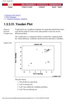
For this sample plot, there are seven factors and each factor has two
levels. For each factor, we define a distinct x coordinate for each level
of the factor. For example, for factor 1, level 1 is coded as 0.8 and level
2 is coded as 1.2. The y coordinate is simply the value of the response

variable. The solid horizontal line is drawn at the overall mean of the
response variable. The vertical dotted lines are added for clarity.
Although the plot can be drawn with an arbitrary number of levels for a
factor, it is really only useful when there are two or three levels for a
factor.
Conclusions This sample dex scatter plot shows that:
there does not appear to be any outliers;1.
the levels of factors 2 and 4 show distinct location differences;
and
2.
the levels of factor 1 show distinct scale differences.3.
Definition:
Response
Values
Versus
Factor
Variables
Dex scatter plots are formed by:
Vertical axis: Value of the response variable
●
Horizontal axis: Factor variable (with each level of the factor
coded with a slightly offset x coordinate)
●
1.3.3.11. DEX Scatter Plot
(2 of 5) [5/1/2006 9:56:36 AM]
Questions The dex scatter plot can be used to answer the following questions:
Which factors are important with respect to location and scale?1.
Are there outliers?2.
Importance:
Identify

Important
Factors with
Respect to
Location and
Scale
The goal of many designed experiments is to determine which factors
are important with respect to location and scale. A ranked list of the
important factors is also often of interest. Dex scatter, mean, and
standard deviation plots show this graphically. The dex scatter plot
additionally shows if outliers may potentially be distorting the results.
Dex scatter plots were designed primarily for analyzing designed
experiments. However, they are useful for any type of multi-factor data
(i.e., a response variable with 2 or more factor variables having a small
number of distinct levels) whether or not the data were generated from
a designed experiment.
Extension for
Interaction
Effects
Using the concept of the scatterplot matrix, the dex scatter plot can be
extended to display first order interaction effects.
Specifically, if there are k factors, we create a matrix of plots with k
rows and k columns. On the diagonal, the plot is simply a dex scatter
plot with a single factor. For the off-diagonal plots, we multiply the
values of X
i
and X
j
. For the common 2-level designs (i.e., each factor
has two levels) the values are typically coded as -1 and 1, so the
multiplied values are also -1 and 1. We then generate a dex scatter plot

for this interaction variable. This plot is called a dex interaction effects
plot and an example is shown below.
1.3.3.11. DEX Scatter Plot
(3 of 5) [5/1/2006 9:56:36 AM]
Interpretation
of the Dex
Interaction
Effects Plot
We can first examine the diagonal elements for the main effects. These
diagonal plots show a great deal of overlap between the levels for all
three factors. This indicates that location and scale effects will be
relatively small.
We can then examine the off-diagonal plots for the first order
interaction effects. For example, the plot in the first row and second
column is the interaction between factors X1 and X2. As with the main
effect plots, no clear patterns are evident.
Related
Techniques
Dex mean plot
Dex standard deviation plot
Block plot
Box plot
Analysis of variance
Case Study
The dex scatter plot is demonstrated in the ceramic strength data case
study.
Software Dex scatter plots are available in some general purpose statistical
software programs, although the format may vary somewhat between
these programs. They are essentially just scatter plots with the X
variable defined in a particular way, so it should be feasible to write

macros for dex scatter plots in most statistical software programs.
Dataplot supports a dex scatter plot.
1.3.3.11. DEX Scatter Plot
(4 of 5) [5/1/2006 9:56:36 AM]
1.3.3.11. DEX Scatter Plot
(5 of 5) [5/1/2006 9:56:36 AM]
factor 7 is the fourth most important;4.
factor 6 is the fifth most important;5.
factors 3 and 5 are relatively unimportant.6.
In summary, factors 4, 2, and 1 seem to be clearly important, factors 3
and 5 seem to be clearly unimportant, and factors 6 and 7 are borderline
factors whose inclusion in any subsequent models will be determined by
further analyses.
Definition:
Mean
Response
Versus
Factor
Variables
Dex mean plots are formed by:
Vertical axis: Mean of the response variable for each level of the
factor
●
Horizontal axis: Factor variable●
Questions The dex mean plot can be used to answer the following questions:
Which factors are important? The dex mean plot does not provide
a definitive answer to this question, but it does help categorize
factors as "clearly important", "clearly not important", and
"borderline importance".
1.

What is the ranking list of the important factors?2.
Importance:
Determine
Significant
Factors
The goal of many designed experiments is to determine which factors
are significant. A ranked order listing of the important factors is also
often of interest. The dex mean plot is ideally suited for answering these
types of questions and we recommend its routine use in analyzing
designed experiments.
Extension
for
Interaction
Effects
Using the concept of the scatter plot matrix, the dex mean plot can be
extended to display first-order interaction effects.
Specifically, if there are k factors, we create a matrix of plots with k
rows and k columns. On the diagonal, the plot is simply a dex mean plot
with a single factor. For the off-diagonal plots, measurements at each
level of the interaction are plotted versus level, where level is X
i
times
X
j
and X
i
is the code for the ith main effect level and X
j
is the code for
the jth main effect. For the common 2-level designs (i.e., each factor has

two levels) the values are typically coded as -1 and 1, so the multiplied
values are also -1 and 1. We then generate a dex mean plot for this
interaction variable. This plot is called a dex interaction effects plot and
an example is shown below.
1.3.3.12. DEX Mean Plot
(2 of 3) [5/1/2006 9:56:36 AM]
DEX
Interaction
Effects Plot
This plot shows that the most significant factor is X1 and the most
significant interaction is between X1 and X3.
Related
Techniques
Dex scatter plot
Dex standard deviation plot
Block plot
Box plot
Analysis of variance
Case Study The dex mean plot and the dex interaction effects plot are demonstrated
in the ceramic strength data case study.
Software Dex mean plots are available in some general purpose statistical
software programs, although the format may vary somewhat between
these programs. It may be feasible to write macros for dex mean plots in
some statistical software programs that do not support this plot directly.
Dataplot supports both a dex mean plot and a dex interaction effects
plot.
1.3.3.12. DEX Mean Plot
(3 of 3) [5/1/2006 9:56:36 AM]
factor 1 has the greatest difference in standard deviations between
factor levels;

1.
factor 4 has a significantly lower average standard deviation than
the average standard deviations of other factors (but the level 1
standard deviation for factor 1 is about the same as the level 1
standard deviation for factor 4);
2.
for all factors, the level 1 standard deviation is smaller than the
level 2 standard deviation.
3.
Definition:
Response
Standard
Deviations
Versus
Factor
Variables
Dex standard deviation plots are formed by:
Vertical axis: Standard deviation of the response variable for each
level of the factor
●
Horizontal axis: Factor variable●
Questions The dex standard deviation plot can be used to answer the following
questions:
How do the standard deviations vary across factors?1.
How do the standard deviations vary within a factor?2.
Which are the most important factors with respect to scale?3.
What is the ranked list of the important factors with respect to
scale?
4.
Importance:

Assess
Variability
The goal with many designed experiments is to determine which factors
are significant. This is usually determined from the means of the factor
levels (which can be conveniently shown with a dex mean plot). A
secondary goal is to assess the variability of the responses both within a
factor and between factors. The dex standard deviation plot is a
convenient way to do this.
Related
Techniques
Dex scatter plot
Dex mean plot
Block plot
Box plot
Analysis of variance
Case Study
The dex standard deviation plot is demonstrated in the ceramic strength
data case study.
1.3.3.13. DEX Standard Deviation Plot
(2 of 3) [5/1/2006 9:56:36 AM]
Software Dex standard deviation plots are not available in most general purpose
statistical software programs. It may be feasible to write macros for dex
standard deviation plots in some statistical software programs that do
not support them directly. Dataplot supports a dex standard deviation
plot.
1.3.3.13. DEX Standard Deviation Plot
(3 of 3) [5/1/2006 9:56:36 AM]
Definition The most common form of the histogram is obtained by splitting the
range of the data into equal-sized bins (called classes). Then for each
bin, the number of points from the data set that fall into each bin are

counted. That is
Vertical axis: Frequency (i.e., counts for each bin)
●
Horizontal axis: Response variable●
The classes can either be defined arbitrarily by the user or via some
systematic rule. A number of theoretically derived rules have been
proposed by Scott (Scott 1992).
The cumulative histogram is a variation of the histogram in which the
vertical axis gives not just the counts for a single bin, but rather gives
the counts for that bin plus all bins for smaller values of the response
variable.
Both the histogram and cumulative histogram have an additional variant
whereby the counts are replaced by the normalized counts. The names
for these variants are the relative histogram and the relative cumulative
histogram.
There are two common ways to normalize the counts.
The normalized count is the count in a class divided by the total
number of observations. In this case the relative counts are
normalized to sum to one (or 100 if a percentage scale is used).
This is the intuitive case where the height of the histogram bar
represents the proportion of the data in each class.
1.
The normalized count is the count in the class divided by the
2.
1.3.3.14. Histogram
(2 of 4) [5/1/2006 9:56:37 AM]
number of observations times the class width. For this
normalization, the area (or integral) under the histogram is equal
to one. From a probabilistic point of view, this normalization
results in a relative histogram that is most akin to the probability

density function and a relative cumulative histogram that is most
akin to the cumulative distribution function. If you want to
overlay a probability density or cumulative distribution function
on top of the histogram, use this normalization. Although this
normalization is less intuitive (relative frequencies greater than 1
are quite permissible), it is the appropriate normalization if you
are using the histogram to model a probability density function.
Questions The histogram can be used to answer the following questions:
What kind of population distribution do the data come from?1.
Where are the data located?2.
How spread out are the data?3.
Are the data symmetric or skewed?4.
Are there outliers in the data?5.
Examples
Normal1.
Symmetric, Non-Normal, Short-Tailed2.
Symmetric, Non-Normal, Long-Tailed3.
Symmetric and Bimodal4.
Bimodal Mixture of 2 Normals5.
Skewed (Non-Symmetric) Right6.
Skewed (Non-Symmetric) Left7.
Symmetric with Outlier8.
Related
Techniques
Box plot
Probability plot
The techniques below are not discussed in the Handbook. However,
they are similar in purpose to the histogram. Additional information on
them is contained in the Chambers and Scott references.
Frequency Plot

Stem and Leaf Plot
Density Trace
Case Study
The histogram is demonstrated in the heat flow meter data case study.
1.3.3.14. Histogram
(3 of 4) [5/1/2006 9:56:37 AM]
Software Histograms are available in most general purpose statistical software
programs. They are also supported in most general purpose charting,
spreadsheet, and business graphics programs. Dataplot supports
histograms.
1.3.3.14. Histogram
(4 of 4) [5/1/2006 9:56:37 AM]
1.3.3.14.1. Histogram Interpretation: Normal
(2 of 2) [5/1/2006 9:56:37 AM]
Description of
What
Short-Tailed
Means
For a symmetric distribution, the "body" of a distribution refers to the
"center" of the distribution commonly that region of the distribution
where most of the probability resides the "fat" part of the distribution.
The "tail" of a distribution refers to the extreme regions of the
distribution both left and right. The "tail length" of a distribution is a
term that indicates how fast these extremes approach zero.
For a short-tailed distribution, the tails approach zero very fast. Such
distributions commonly have a truncated ("sawed-off") look. The
classical short-tailed distribution is the uniform (rectangular)
distribution in which the probability is constant over a given range and
then drops to zero everywhere else we would speak of this as having
no tails, or extremely short tails.

For a moderate-tailed distribution, the tails decline to zero in a
moderate fashion. The classical moderate-tailed distribution is the
normal (Gaussian) distribution.
For a long-tailed distribution, the tails decline to zero very slowly and
hence one is apt to see probability a long way from the body of the
distribution. The classical long-tailed distribution is the Cauchy
distribution.
In terms of tail length, the histogram shown above would be
characteristic of a "short-tailed" distribution.
The optimal (unbiased and most precise) estimator for location for the
center of a distribution is heavily dependent on the tail length of the
distribution. The common choice of taking N observations and using
the calculated sample mean as the best estimate for the center of the
distribution is a good choice for the normal distribution (moderate
tailed), a poor choice for the uniform distribution (short tailed), and a
horrible choice for the Cauchy distribution (long tailed). Although for
the normal distribution the sample mean is as precise an estimator as
we can get, for the uniform and Cauchy distributions, the sample mean
is not the best estimator.
For the uniform distribution, the midrange
midrange = (smallest + largest) / 2
is the best estimator of location. For a Cauchy distribution, the median
is the best estimator of location.
Recommended
Next Step
If the histogram indicates a symmetric, short-tailed distribution, the
recommended next step is to generate a uniform probability plot. If the
uniform probability plot is linear, then the uniform distribution is an
appropriate model for the data.
1.3.3.14.2. Histogram Interpretation: Symmetric, Non-Normal, Short-Tailed

(2 of 3) [5/1/2006 9:56:37 AM]
1.3.3.14.2. Histogram Interpretation: Symmetric, Non-Normal, Short-Tailed
(3 of 3) [5/1/2006 9:56:37 AM]
Recommended
Next Step
If the histogram indicates a symmetric, long tailed distribution, the
recommended next step is to do a Cauchy probability plot. If the
Cauchy probability plot is linear, then the Cauchy distribution is an
appropriate model for the data. Alternatively, a Tukey Lambda PPCC
plot may provide insight into a suitable distributional model for the
data.
1.3.3.14.3. Histogram Interpretation: Symmetric, Non-Normal, Long-Tailed
(2 of 2) [5/1/2006 9:56:38 AM]
improved deterministic modeling of the phenomenon under study. For
example, for the data presented above, the bimodal histogram is
caused by sinusoidality in the data.
Recommended
Next Step
If the histogram indicates a symmetric, bimodal distribution, the
recommended next steps are to:
Do a run sequence plot or a scatter plot to check for
sinusoidality.
1.
Do a lag plot to check for sinusoidality. If the lag plot is
elliptical, then the data are sinusoidal.
2.
If the data are sinusoidal, then a spectral plot is used to
graphically estimate the underlying sinusoidal frequency.
3.
If the data are not sinusoidal, then a Tukey Lambda PPCC plot

may determine the best-fit symmetric distribution for the data.
4.
The data may be fit with a mixture of two distributions. A
common approach to this case is to fit a mixture of 2 normal or
lognormal distributions. Further discussion of fitting mixtures of
distributions is beyond the scope of this Handbook.
5.
1.3.3.14.4. Histogram Interpretation: Symmetric and Bimodal
(2 of 2) [5/1/2006 9:56:38 AM]