Engineering Statistics Handbook Episode 3 Part 13 pdf

2. Measurement Process Characterization
2.3. Calibration
2.3.4. Catalog of calibration designs
2.3.4.5. Designs for angle blocks
2.3.4.5.3.Design for 6 angle blocks
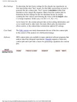
DESIGN MATRIX
1 1 1 1 1 1

0 1 -1 0 0 0
-1 1 0 0 0 0
0 1 0 -1 0 0
0 -1 0 0 0 1
-1 0 0 0 0 1
0 0 -1 0 0 1
0 0 0 0 1 -1
-1 0 0 0 1 0
0 -1 0 0 1 0
0 0 0 1 -1 0
-1 0 0 1 0 0
0 0 0 1 0 -1
0 0 1 -1 0 0
-1 0 1 0 0 0
0 0 1 0 -1 0

REFERENCE +
CHECK STANDARD +

DEGREES OF FREEDOM = 10
SOLUTION MATRIX
DIVISOR = 24

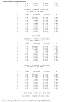
OBSERVATIONS 1 1 1 1 1
2.3.4.5.3. Design for 6 angle blocks
(1 of 3) [5/1/2006 10:12:19 AM]
1
Y(11) 0.0000 3.2929 -5.2312 -0.7507 -0.6445
-0.6666
Y(12) 0.0000 6.9974 4.6324 4.6495 3.8668
3.8540
Y(13) 0.0000 3.2687 -0.7721 -5.2098 -0.6202
-0.6666
Y(21) 0.0000 -5.2312 -0.7507 -0.6445 -0.6666
3.2929
Y(22) 0.0000 4.6324 4.6495 3.8668 3.8540
6.9974
Y(23) 0.0000 -0.7721 -5.2098 -0.6202 -0.6666
3.2687
Y(31) 0.0000 -0.7507 -0.6445 -0.6666 3.2929
-5.2312
Y(32) 0.0000 4.6495 3.8668 3.8540 6.9974
4.6324
Y(33) 0.0000 -5.2098 -0.6202 -0.6666 3.2687
-0.7721
Y(41) 0.0000 -0.6445 -0.6666 3.2929 -5.2312
-0.7507
Y(42) 0.0000 3.8668 3.8540 6.9974 4.6324
4.6495
Y(43) 0.0000 -0.6202 -0.6666 3.2687 -0.7721
-5.2098
Y(51) 0.0000 -0.6666 3.2929 -5.2312 -0.7507
-0.6445

Y(52) 0.0000 3.8540 6.9974 4.6324 4.6495
3.8668
Y(53) 0.0000 -0.6666 3.2687 -0.7721 -5.2098
-0.6202
R* 1. 1. 1. 1. 1.
1.
R* = VALUE OF REFERENCE ANGLE BLOCK
FACTORS FOR REPEATABILITY STANDARD DEVIATIONS
SIZE K1
1 1 1 1 1 1
1 0.0000 +
1 0.7111 +
1 0.7111 +
1 0.7111 +
1 0.7111 +
2.3.4.5.3. Design for 6 angle blocks
(2 of 3) [5/1/2006 10:12:19 AM]
1 0.7111 +
1 0.7111 +
Explanation of notation and interpretation of tables
2.3.4.5.3. Design for 6 angle blocks
(3 of 3) [5/1/2006 10:12:19 AM]
Estimates of
drift
The estimates of the shift due to the resistance thermometer and
temperature drift are given by:
Standard
deviations
The residual variance is given by
.

The standard deviation of the indication assigned to the ith test
thermometer is
and the standard deviation for the estimates of shift and drift are
respectively.
2.3.4.6. Thermometers in a bath
(2 of 2) [5/1/2006 10:12:20 AM]
2. Measurement Process Characterization
2.3. Calibration
2.3.4. Catalog of calibration designs
2.3.4.7. Humidity standards
2.3.4.7.1.Drift-elimination design for 2
reference weights and 3 cylinders
OBSERVATIONS 1 1 1 1 1
Y(1) + -
Y(2) + -
Y(3) + -
Y(4) + -
Y(5) - +
Y(6) - +
Y(7) + -
Y(8) + -
Y(9) - +
Y(10) + -
RESTRAINT + +
CHECK STANDARD + -
DEGREES OF FREEDOM = 6
SOLUTION MATRIX
DIVISOR = 10
OBSERVATIONS 1 1 1 1 1
2.3.4.7.1. Drift-elimination design for 2 reference weights and 3 cylinders

(1 of 2) [5/1/2006 10:12:20 AM]
Y(1) 2 -2 0 0 0
Y(2) 0 0 0 2 -2
Y(3) 0 0 2 -2 0
Y(4) -1 1 -3 -1 -1
Y(5) -1 1 1 1 3
Y(6) -1 1 1 3 1
Y(7) 0 0 2 0 -2
Y(8) -1 1 -1 -3 -1
Y(9) 1 -1 1 1 3
Y(10) 1 -1 -3 -1 -1
R* 5 5 5 5 5
R* = average value of the two reference weights
FACTORS FOR REPEATABILITY STANDARD DEVIATIONS

WT K1 1 1 1 1 1
1 0.5477 +
1 0.5477 +
1 0.5477 +
2 0.8944 + +
3 1.2247 + + +
0 0.6325 + -
Explanation of notation and interpretation of tables
2.3.4.7.1. Drift-elimination design for 2 reference weights and 3 cylinders
(2 of 2) [5/1/2006 10:12:20 AM]
standards at all nominal lengths.
A check standard can also be a mathematical construction, such as the
computed difference between the calibrated values of two reference
standards in a design.
Database of

check
standard
values
The creation and maintenance of the database of check standard values
is an important aspect of the control process. The results from each
calibration run are recorded in the database. The best way to record this
information is in one file with one line (row in a spreadsheet) of
information in fixed fields for each calibration run. A list of typical
entries follows:
Date1.
Identification for check standard2.
Identification for the calibration design3.
Identification for the instrument4.
Check standard value5.
Repeatability standard deviation from design6.
Degrees of freedom7.
Operator identification8.
Flag for out-of-control signal9.
Environmental readings (if pertinent)10.
2.3.5. Control of artifact calibration
(2 of 2) [5/1/2006 10:12:20 AM]
Control
procedure is
invoked in
real-time for
each
calibration
run
The control procedure compares each new repeatability standard
deviation that is recorded for the instrument with an upper control limit,

UCL. Usually, only the upper control limit is of interest because we are
primarily interested in detecting degradation in the instrument's
precision. A possible complication is that the control limit is dependent
on the degrees of freedom in the new standard deviation and is
computed as follows:
.
The quantity under the radical is the upper
percentage point from the
F table where is chosen small to be, say, 05. The other two terms
refer to the degrees of freedom in the new standard deviation and the
degrees of freedom in the process standard deviation.
Limitation
of graphical
method
The graphical method of plotting every new estimate of repeatability on
a control chart does not work well when the UCL can change with each
calibration design, depending on the degrees of freedom. The algebraic
equivalent is to test if the new standard deviation exceeds its control
limit, in which case the short-term precision is judged to be out of
control and the current calibration run is rejected. For more guidance,
see Remedies and strategies for dealing with out-of-control signals.
As long as the repeatability standard deviations are in control, there is
reason for confidence that the precision of the instrument has not
degraded.
Case study:
Mass
balance
precision
It is recommended that the repeatability standard deviations be plotted
against time on a regular basis to check for gradual degradation in the

instrument. Individual failures may not trigger a suspicion that the
instrument is in need of adjustment or tuning.
2.3.5.1. Control of precision
(2 of 2) [5/1/2006 10:12:21 AM]
let f=sqrt(f)
let sul=f*scc
plot s scc sul vs t
Control chart
for precision
TIME IN YEARS
Interpretation
of the control
chart
The control chart shows that the precision of the balance remained in control through 1990
with only two violations of the control limits. For those occasions, the calibrations were
discarded and repeated. Clearly, for the second violation, something significant occurred
that invalidated the calibration results.
Further
interpretation
of the control
chart
However, it is also clear from the pattern of standard deviations over time that the precision
of the balance was gradually degrading and more and more points were approaching the
control limits. This finding led to a decision to replace this balance for high accuracy
calibrations.
2.3.5.1.1. Example of control chart for precision
(2 of 2) [5/1/2006 10:12:21 AM]
The control
limits depend
on the t-

distribution
and the
degrees of
freedom in the
process
standard
deviation
If
has been computed from historical data, the upper and lower
control limits are:
with denoting the upper critical value from the
t-table with v = (K - 1) degrees of freedom.
Run software
macro for
computing the
t-factor
Dataplot can compute the value of the t-statistic. For a conservative
case with
= 0.05 and K = 6, the commands
let alphau = 1 - 0.05/2
let k = 6
let v1 = k-1
let t = tppf(alphau, v1)
return the following value:
THE COMPUTED VALUE OF THE CONSTANT T =
0.2570583E+01
Simplification
for large
degrees of
freedom

It is standard practice to use a value of 3 instead of a critical value
from the t-table, given the process standard deviation has large degrees
of freedom, say, v > 15.
The control
procedure is
invoked in
real-time and
a failure
implies that
the current
calibration
should be
rejected
The control procedure compares the check standard value,
C, from
each calibration run with the upper and lower control limits. This
procedure should be implemented in real time and does not necessarily
require a graphical presentation. The check standard value can be
compared algebraically with the control limits. The calibration run is
judged to be out-of-control if either:
C > UCL
or
C < LCL
2.3.5.2. Control of bias and long-term variability
(2 of 3) [5/1/2006 10:12:22 AM]
Actions to be
taken
If the check standard value exceeds one of the control limits, the
process is judged to be out of control and the current calibration run is
rejected. The best strategy in this situation is to repeat the calibration

to see if the failure was a chance occurrence. Check standard values
that remain in control, especially over a period of time, provide
confidence that no new biases have been introduced into the
measurement process and that the long-term variability of the process
has not changed.
Out-of-control
signals that
recur require
investigation
Out-of-control signals, particularly if they recur, can be symptomatic
of one of the following conditions:
Change or damage to the reference standard(s)
●
Change or damage to the check standard●
Change in the long-term variability of the calibration process●
For more guidance, see Remedies and strategies for dealing with
out-of-control signals.
Caution - be
sure to plot
the data
If the tests for control are carried out algebraically, it is recommended
that, at regular intervals, the check standard values be plotted against
time to check for drift or anomalies in the measurement process.
2.3.5.2. Control of bias and long-term variability
(3 of 3) [5/1/2006 10:12:22 AM]
let ll=cc-3*sd
characters * blank blank blank * blank blank blank
lines blank solid dotted dotted blank solid dotted dotted
plot y cc ul ll vs t
.end of calculations

Control chart
of
measurements
of kilogram
check standard
showing a
change in the
process after
1985
Interpretation
of the control
chart
The control chart shows only two violations of the control limits. For those occasions, the calibrations
were discarded and repeated. The configuration of points is unacceptable if many points are close to a
control limit and there is an unequal distribution of data points on the two sides of the control chart
indicating a change in either:
process average which may be related to a change in the reference standards
●
or
variability which may be caused by a change in the instrument precision or may be the result of
other factors on the measurement process.
●
Small changes
only become
obvious over
time
Unfortunately, it takes time for the patterns in the data to emerge because individual violations of the
control limits do not necessarily point to a permanent shift in the process. The Shewhart control chart
is not powerful for detecting small changes, say of the order of at most one standard deviation, which
appears to be approximately the case in this application. This level of change might seem

insignificant, but the calculation of uncertainties for the calibration process depends on the control
limits.
2.3.5.2.1. Example of Shewhart control chart for mass calibrations
(2 of 3) [5/1/2006 10:12:22 AM]
Re-establishing
the limits
based on
recent data
and EWMA
option
If the limits for the control chart are re-calculated based on the data after 1985, the extent of the
change is obvious. Because the exponentially weighted moving average (EWMA) control chart is
capable of detecting small changes, it may be a better choice for a high precision process that is
producing many control values.
Run
continuation of
software
macro for
updating
Shewhart
control chart
Dataplot commands for updating the control chart are as follows:
let ybar2=mean y subset t > 85
let sd2=standard deviation y subset t > 85
let n = size y
let cc2=ybar2 for i = 1 1 n
let ul2=cc2+3*sd2
let ll2=cc2-3*sd2
plot y cc ul ll vs t subset t < 85 and
plot y cc2 ul2 ll2 vs t subset t > 85

Revised
control chart
based on check
standard
measurements
after 1985
2.3.5.2.1. Example of Shewhart control chart for mass calibrations
(3 of 3) [5/1/2006 10:12:22 AM]
Example of
EWMA chart
for check
standard data
for kilogram
calibrations
showing
multiple
violations of
the control
limits for the
EWMA
statistics
The target (average) and process standard deviation are computed from the check standard data taken
prior to 1985. The computation of the EWMA statistic begins with the data taken at the start of 1985.
In the control chart below, the control data after 1985 are shown in green, and the EWMA statistics
are shown as black dots superimposed on the raw data. The control limits are calculated according to
the equation above where the process standard deviation, s = 0.03065 mg and k = 3. The EWMA
statistics, and not the raw data, are of interest in looking for out-of-control signals. Because the
EWMA statistic is a weighted average, it has a smaller standard deviation than a single control
measurement, and, therefore, the EWMA control limits are narrower than the limits for a Shewhart
control chart.

Run the
software
macro for
creating the
Shewhart
control chart
Dataplot commands for creating the control chart are as follows:
dimension 500 30
skip 4
read mass.dat x id y bal s ds
let n = number y
let cutoff = 85.0
let tag = 2 for i = 1 1 n
let tag = 1 subset x < cutoff
xlimits 75 90
let m = mean y subset tag 1
let s = sd y subset tag 1
let lambda = .2
let fudge = sqrt(lambda/(2-lambda))
let mean = m for i = 1 1 n
2.3.5.2.2. Example of EWMA control chart for mass calibrations
(2 of 3) [5/1/2006 10:12:22 AM]
let upper = mean + 3*fudge*s
let lower = mean - 3*fudge*s
let nm1 = n-1
let start = 106
let pred2 = mean
loop for i = start 1 nm1
let ip1 = i+1
let yi = y(i)

let predi = pred2(i)
let predip1 = lambda*yi + (1-lambda)*predi
let pred2(ip1) = predip1
end loop
char * blank * circle blank blank
char size 2 2 2 1 2 2
char fill on all
lines blank dotted blank solid solid solid
plot y mean versus x and
plot y pred2 lower upper versus x subset x > cutoff
Interpretation
of the control
chart
The EWMA control chart shows many violations of the control limits starting at approximately the
mid-point of 1986. This pattern emerges because the process average has actually shifted about one
standard deviation, and the EWMA control chart is sensitive to small changes.
2.3.5.2.2. Example of EWMA control chart for mass calibrations
(3 of 3) [5/1/2006 10:12:22 AM]