Engineering Analysis with Ansys Software Episode 2 Part 6 pptx

Ch06-H6875.tex 24/11/2006 17: 48 page 284
284 Chapter 6 Application of ANSYS to thermo mechanics
A
B
Figure 6.36 On Working Plane (path name: AB).
A
C
B
Figure 6.37 Map Result Items onto Path (AB path).
Ch06-H6875.tex 24/11/2006 17: 48 page 285
6.3 Steady-state thermal analysis of a pipe intersection 285
A
C
B
Figure 6.38 Map Result Items onto Path (AB path).
A
B
Figure 6.39 Plot of Path Items on Graph.
6.3
Steady-state thermal analysis of a
pipe intersection
6.3.1 Description of the problem
A cylindrical tank is penetrated radially by a small pipe at a point on its axis remote
from the ends of the tank, as shown in Figure 6.41.
Ch06-H6875.tex 24/11/2006 17: 48 page 286
286 Chapter 6 Application of ANSYS to thermo mechanics
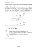
Figure 6.40 Variations of temperature gradients along path AB.
Figure 6.41 Pipe intersection.
The inside of the tank is exposed to a fluid with temperature of 232
◦
C. The

pipe experiences a steady flow of fluid with temperature of 38
◦
C, and the two flow
regimes are isolated from each other by means of a thin tube. The convection (film)
coefficient in the pipe varies with the metal temperature and is thus expressed as a
Ch06-H6875.tex 24/11/2006 17: 48 page 287
6.3 Steady-state thermal analysis of a pipe intersection 287
material property. The objective is to determine the temperature distribution at the
pipe–tank junction.
The following data describing the problem are given:
•
Inside diameter of the pipe =8mm
•
Outside diameter of the pipe =10 mm
•
Inside diameter of the tank =26 mm
•
Outside diameter of the tank =30 mm
•
Inside bulk fluid temperature, tank =232
◦
C
•
Inside convection coefficient, tank =4.92 W/m
2 ◦
C
•
Inside bulk fluid temperature, pipe =38
◦
C

•
Inside convection coefficient (pipe) varies from about 19.68 to 39.36 W/m
2 ◦
C,
depending on temperature.
Table 6.1 provides information about variation of the thermal parameters with
temperature.
Table 6.1 Variation of the thermal parameters with temperature
Temperature [
◦
C] 21 93 149 204 260
Convection coefficient 41.918 39.852 34.637 27.06 21.746
[W/m
2 ◦
C]
Density [kg/m
3
] 7889 7889 7889 7889 7889
Conductivity 0.2505 0.267 0.2805 0.294 0.3069
[J/s m
◦
C]
Specific heat 6.898 7.143 7.265 7.448 7.631
[J/kg
◦
C]
The assumption is made that the quarter symmetry is applicable and that, at the
terminus of the model (longitudinal and circumferential cuts in the tank), there
is sufficient attenuation of the pipe effects such that these edges can be held at
232

◦
C.
The solid model is constructed by intersecting the tank with the pipe and then
removing the internal part of the pipe using Boolean operation.
Boundary temperatures along with the convection coefficients and bulk fluid
temperatures are dealt with in the solution phase, after which a static solution is
executed.
Temperature contours and thermal flux displays are obtained in postprocessing.
Details of steps taken to create the model of pipe intersecting with tank are
outlined below.
Ch06-H6875.tex 24/11/2006 17: 48 page 288
288 Chapter 6 Application of ANSYS to thermo mechanics
6.3.2 Preparation for model building
From ANSYS Main Menu select Preferences. This frame is shown in Figure 6.42.
A
Figure 6.42 Preferences: Thermal.
Depending on the nature of analysis to be attempted an appropriate analysis type
should be selected. In the problem considered here [A] Thermal was selected as
shown in Figure 6.42.
From ANSYS Main Menu select Preprocessor and then Element Type and
Add/Edit/Delete. The frame shown in Figure 6.43 appears.
Clicking [A] Add button activates a new set of options which are shown in
Figure 6.44.
Figure 6.44 indicates that for the problem considered here the following was
selected: [A] Thermal Mass →Solid and [B] 20node 90.
From ANSYS Main Menu select Material Props and then Material Models.
Figure 6.45 shows the resulting frame.
From the options listed on the right hand select [A] Thermal as shown in
Figure 6.45.
Next select [B] Conductivity, Isotropic. The frame shown in Figure 6.46 appears.

Ch06-H6875.tex 24/11/2006 17: 48 page 289
6.3 Steady-state thermal analysis of a pipe intersection 289
A
Figure 6.43 Element Types selection.
A
B
Figure 6.44 Library of Element Types.
Then, using conductivity versus temperature values, listed in Table 6.1, appropri-
ate figures should be typed in as shown in Figure 6.46.
By selecting [C] Specific Heat option on the right-hand column (see Figure 6.45),
the frame shown in Figure 6.47 is produced.
Appropriate values of specific heat versus temperature, taken from Table 6.1, are
typed as shown in Figure 6.47.
The next material property to be defined is density. According to Table 6.1,
density is constant for all temperatures used. Therefore, selecting [D] Density
Ch06-H6875.tex 24/11/2006 17: 48 page 290
290 Chapter 6 Application of ANSYS to thermo mechanics
A
C
E
D
B
Figure 6.45 Define Material Model Behavior.
Figure 6.46 Conductivity for Material Number 1.
from the right-hand column (see Figure 6.45), results in the frame shown in
Figure 6.48.
Density of 7888.8 kg/m
3
is typed in the box shown in Figure 6.48.
All the above properties were used to characterize Material Number 1. Convection

or film coefficient is another important parameter characterizing the system being
analyzed. However, it is not a property belonging to Material Number 1 (material of
the tank and pipe) but to a thin film formed by the liquid on solid surfaces. It is a
different entity and, therefore, is called Material Number 2.
Ch06-H6875.tex 24/11/2006 17: 48 page 291
6.3 Steady-state thermal analysis of a pipe intersection 291
Figure 6.47 Specific Heat for Material Number 1.
Figure 6.48 Density for Material Number 1.
Selecting [E] Convection or Film Coef. (see Figure 6.45) results in the frame
shown in Figure 6.49. Appropriate values of film coefficient for various temperatures,
taken from Table 6.1, are introduced as shown in Figure 6.49.
6.3.3 Construction of the model
The entire model of the pipe intersecting with the tank is constructed using one of
the three-dimensional (3D) primitive shapes, that is cylindrical. Only one-quarter of
Ch06-H6875.tex 24/11/2006 17: 48 page 292
292 Chapter 6 Application of ANSYS to thermo mechanics
Figure 6.49 Convection or Film Coefficient for Material Number 2.
the tank–pipe assembly will be sufficient to use in the analysis. From ANSYS Main
Menu select Preprocessor → Modelling →Create →Volumes →Cylinder →By
Dimensions. Figure 6.50 shows the resulting frame.
A
B
D
F
C
E
Figure 6.50 Create Cylinder by Dimensions.
In Figure 6.50, as shown, the following inputs are made: [A] RAD1 =1.5 cm; [B]
RAD2 =1.3 cm; [C] Z1 =0; [D] Z2 =2 cm; [E] THETA1=0; [F] THETA2=90.
As the pipe axis is at right angle to the cylinder axis, therefore it is necessary to

rotate the working plane (WP) to the pipe axis by 90
◦
. This is done by selecting from
Utility Menu WorkPlane →Offset WP by Increments. The resulting frame is shown
in Figure 6.51.
Ch06-H6875.tex 24/11/2006 17: 48 page 293
6.3 Steady-state thermal analysis of a pipe intersection 293
A
Figure 6.51 Offset WP by Increments.
In Figure 6.51, the input is shown as [A] XY =0; YZ =−90 and the ZX is left
unchanged from default value. Next, from ANSYSMainMenu selectPreprocessor →
Modelling →Create →Volumes →Cylinder →By Dimensions. Figure 6.52 shows
the resulting frame.
Ch06-H6875.tex 24/11/2006 17: 48 page 294
294 Chapter 6 Application of ANSYS to thermo mechanics
A
C
B
D
F
E
Figure 6.52 Create Cylinder by Dimensions.
A
Figure 6.53 Overlap Volumes (Booleans Operation).
In Figure 6.52, as shown, the following
inputs are made: [A] RAD1 =0.5 cm; [B]
RAD2 =0.4 cm; [C] Z1 =0; [D] Z2 =2 cm;
[E] THETA1=0; [F] THETA2=−90.
After that the WP should be set to the
default setting by inputting in Figure 6.51

YZ =90 this time.As the cylinderandthe pipe
are separate entities, it is necessary to overlap
them in order to make the one component.
From ANSYS Main Menu select Preproces-
sor → Modelling → Create → Operate →
Booleans →Overlap →Volumes. The frame
shown in Figure 6.53 is created.
Pick both elements, that is cylinder and
pipe, and press [A] OK buttontoexecute
the selection. Next activate volume number-
ing which will be of help when carrying out
further operations on volumes. This is done
by selecting from Utility Menu PlotCtrls →
Numbering and checking, in the resulting
frame, VOLU option.
Finally, 3D view of the model should be
set by selecting from Utility Menu the follow-
ing: PlotCtrls →View Settings. The resulting
frame is shown in Figure 6.54.
The following inputs should be made (see
Figure 6.54): [A] XV =−3; [B]YV =−1; [C]
ZV =1 in order to plot the model as shown in Figure 6.55. However, this is not the
only possible view of the model and any other preference may be chosen.
Ch06-H6875.tex 24/11/2006 17: 48 page 295
6.3 Steady-state thermal analysis of a pipe intersection 295
B
A
C
Figure 6.54 View Settings.
Figure 6.55 Quarter symmetry model of the tank–pipe intersection.

Certain volumes of the models, shown in Figure 6.55, are redundant and should
be deleted. FromANSYSMain Menu select Preprocessor →Modelling →Delete →
Volume and Below. Figure 6.56 shows the resulting frame.
VolumesV4 and V3 (acorner of the cylinder) shouldbe picked and [A] OK button
pressed to implement the selection. After the delete operation, the model looks like
that shown in Figure 6.57.
Ch06-H6875.tex 24/11/2006 17: 48 page 296
296 Chapter 6 Application of ANSYS to thermo mechanics
A
Figure 6.56 Delete Volume and Below.
Figure 6.57 Quarter symmetry model of the tank–pipe intersection.
Ch06-H6875.tex 24/11/2006 17: 48 page 297
6.3 Steady-state thermal analysis of a pipe intersection 297
Finally, volumes V5, V6, and V7 should be added in order to create a single vol-
ume required for further analysis. From ANSYS Main Menu select Preprocessor →
Modelling → Operate → Booleans → Add → Volumes. The resulting frame asks
for picking volumes to be added. Pick all three volumes, that is V5, V6, and V7, and
click OK button to implement the operation. Figure 6.58 shows the model of the pipe
intersecting the cylinder as one volume V1.
Figure 6.58 Quarter symmetry model of the tank–pipe intersection represented by a single volume V1.
Meshing of the model usually begins with setting size of elements to be used.
From ANSYS Main Menu select Meshing → Size Cntrls →SmartSize → Basic.A
frame shown in Figure 6.59 appears.
A
B
Figure 6.59 Basic SmartSize Settings.
Ch06-H6875.tex 24/11/2006 17: 48 page 298
298 Chapter 6 Application of ANSYS to thermo mechanics
For the case considered, [A] Size Level – 1 (fine) was selected as shown in Fig-
ure 6.59. Clicking [B] OK button implements the selection. Next, from ANSYS Main

Menu select Mesh → Volumes → Free. The frame shown in Figure 6.60 appears.
Select the volume to be meshed and click [A] OK button.
The resulting network of elements is shown in Figure 6.61.
A
Figure 6.60 Mesh Volumes frame.
Figure 6.61 Meshed quarter symmetry model of
the tank–pipe intersection.
6.3.4 Solution
The meshing operation ends the model construction and the Preprocessor stage.
The solution stage can now be started. From ANSYS Main Menu select Solution →
Analysis Type →New Analysis. Figure 6.62 shows the resulting frame.
Activate [A] Steady-State button. Next, select Solution → Analysis Type →
Analysis Options. In the resulting frame, shown in Figure 6.63, select [A] Program
chosen option.
Ch06-H6875.tex 24/11/2006 17: 48 page 299
6.3 Steady-state thermal analysis of a pipe intersection 299
A
Figure 6.62 New Analysis window.
A
Figure 6.63 Analysis Options.
In order to set starting temperature of 232
◦
CatallnodesselectSolution →
Define Loads →Apply →Thermal →Temperature →Uniform Temp. Figure 6.64
shows the resulting frame. Input [A] Uniform temperature =232
◦
C as shown in
Figure 6.64.
From Utility Menu select WorkPlane → Change Active CS to → Specified
Coord Sys. As a result of that the frame shown in Figure 6.65 appears.

Ch06-H6875.tex 24/11/2006 17: 48 page 300
300 Chapter 6 Application of ANSYS to thermo mechanics
A
Figure 6.64 Temperature selection.
A
B
Figure 6.65 Change Coordinate System.
In order to re-establish a cylindrical coordinate system with Z as the axis of
rotation select [A] Coordinate system number =1 and press [B] OK button to
implement the selection.
Nodes on inner surface of the tank ought to be selected to apply surface loads to
them. The surface load relevant in this case is convection load acting on all nodes
located on inner surface of the tank. From Utility Menu select Select → Entities.
The frame shown in Figure 6.66 appears.
From the first pull down menu select [A] Nodes, from the second pull down
menu select [B] By Location. Also, activate [C] X coordinates button and enter [D]
Min,Max =1.3 (inside radius of the tank). All the four required steps are shown in
Figure 6.66. When the subset of nodes on inner surface of the tank is selected then
the convection load at all nodes has to be applied. From ANSYS Main Menu select
Solution →Define Load → Apply → Thermal → Convection → On nodes.The
resulting frame is shown in Figure 6.67.
Press [A] Pick All in order to call up another frame shown in Figure 6.68.
Inputs into the frame of Figure 6.68 are shown as: [A] Film coefficient =4.92
and [B] Bulk temperature =232. Both quantities are taken from Table 6.1.
From Utility Menu select Select → Entities in order to select a subset of nodes
located at the far edge of the tank. The frame shown in Figure 6.69 appears.
From the first pull down menu select [A] Nodes, from the second pull down
menu select [B] By Location. Also, activate [C] Z coordinates button and [D] enter
Min,Max =2 (the length of the tank in Z-direction). All the four required steps are
Ch06-H6875.tex 24/11/2006 17: 48 page 301

6.3 Steady-state thermal analysis of a pipe intersection 301
A
B
C
D
Figure 6.66 Select Entities.
A
Figure 6.67 Apply Thermal Con-
vection on Nodes.
A
B
Figure 6.68 Select All Nodes.
Ch06-H6875.tex 24/11/2006 17: 48 page 302
302 Chapter 6 Application of ANSYS to thermo mechanics
A
B
C
D
Figure 6.69 Select Entities.
A
Figure 6.70 Select All Nodes.
shown in Figure 6.69. Next, constraints at nodes located at the far edge of the tank
(additional subset of nodes just selected) have to be applied. From ANSYS Main
Menu select Solution → Define Loads → Apply → Thermal → Temperature →
On Nodes. The frame shown in Figure 6.70 appears.
Click [A] Pick All as shown in Figure 6.70. This action brings another frame
shown in Figure 6.71.
Activate both [A] All DOF and TEMP and input [B] TEMP value =232
◦
Cas

shown in Figure 6.71. Finally, click [C] OK to apply temperature constraints on
nodes at the far edge of the tank. The steps outlined above should be followed to
apply constraints at nodes located at the bottom of the tank. From Utility Menu
select Select →Entities. The frame shown in Figure 6.72 appears.
From the first pull down menu select [A] Nodes, from the second pull down
menu select [B] By Location. Also, activate [C] Y coordinates button and [D] enter
Min,Max =0 (location of the bottom of the tankinY-direction). Allthe fourrequired
steps are shown in Figure 6.72. Next, constraints at nodes located at the bottom
of the tank (additional subset of nodes selected above) have to be applied. From
ANSYS Main Menu select Solution → Define Loads → Apply → Thermal →
Temperature → On Nodes. The frame shown in Figure 6.70 appears. As shown in
Ch06-H6875.tex 24/11/2006 17: 48 page 303
6.3 Steady-state thermal analysis of a pipe intersection 303
A
B
C
Figure 6.71 Apply Temperature to All Nodes.
A
B
C
D
Figure 6.72 Select Entities.