HPLC for Food Analysis phần 7 pot
Bạn đang xem bản rút gọn của tài liệu. Xem và tải ngay bản đầy đủ của tài liệu tại đây (548.63 KB, 14 trang )
73
Derivatization
Sample
Reagent
Metering
device
Sampling
unit
6-port valve
Reagent
To waste
From pump
To column
Figure 47
Automated precolumn derivatization
The robotic arm of the autosampler transports, in turn, a
sample vial and several reaction vials under the injection
needle. The needle is extended by a length of capillary at
the point at which the derivatization reaction takes place.
As discussed later in chapter 8, derivatization may be
required if the analytes lack chromophores and if detection
is not sensitive enough. In this process, a chromophore
group is added using a derivatization reagent. Derivatization
can occur either in front of or behind the analytical column
and is used to improve sensitivity and/or selectivity.
Precolumn derivatization is preferable because it requires
no additional reagent pump and because reagents can be
apportioned to each sample rather than pumped through
continuously. Automated precolumn derivatization yields
excellent precision. Moreover, it can handle volumes in the
microliter range, which is especially important when
sample volume is limited. The principles involved are
illustrated in figure 47.
74
The injector draws distinct plugs of sample and derivatization
reagent into the capillary. The back-and-forth movement
of the plunger mixes the plugs. With the right software, the
autoinjector can be paused for a specified length of time to
allow the reaction to proceed to completion. If the reaction
requires several reagents, the autosampler must be
programmable, that is, it must be able to draw sequentially
from different reagent vials into one capillary.
In this complex sample manipulation, the needle must be
cleaned between vials, for example by dipping into wash
vials of distilled water.
Automated sampling systems offer significant advantages
over manual injectors, the most important of which is
higher reproducibility of the injection volume. Sample
throughput also can be increased dramatically. Modern
autosamplers are designed for online sample preparation
and derivatization. For food analysis, an automated
injection system is the best choice.
In brief…
6
Chapter 7
Mobile phase
pumps and
degassers
Characteristics of a
modern HPLC pump
Flow ranges
Gradient elution
The pump is the most critical piece of equipment for
successful HPLC. Performance depends strongly on
the flow behavior of the solvent mixture used as
mobile phase—varying solvent flow rates result in
varying retention times and areas. Conclusions
from a calibration run for peak identification or
quantification depend on reproducible data. In this
chapter we discuss multiple aspects of pump
operation, including solvent pretreatment and its
effect on performance.
A modern HPLC pump must have pulse-free flow, high
precision of the flow rates set, a wide flow rate range, and
low dead volume. In addition, it must exhibit control of a
maximum operating pressure and of at least two solvent
sources for mobile-phase gradients, as well as precision and
accuracy in mixing composition for these gradients.
We discuss two gradient pump types: that constructed for
flow rates between 0.2 and 10 ml/min (low-pressure gradient
formation), and that designed for flow rates between 0.05
and 5 ml/min (high-pressure gradient formation).
In separating the multiple constituents of a typical food
sample, HPLC column selectivity with a particular mobile
phase is not sufficient to resolve every peak. Changing the
eluant strength over the course of the elution by mixing
increasing proportions of a second or third solvent in the
flow path above the column improves peak resolution in two
76
7
77
ways. First, resolution is improved without extending the
elution period, which prevents long retention times (peaks
that have been retained on the column for a longer period of
time tend to broaden and flatten through diffusion, lowering
the S/N and therefore detection levels). Second, gradient
elution sharpens peak widths and shortens run time,
enabling more samples to be analyzed within a given time
frame. The solvents that form the gradient in front of the
column can be mixed either after the pump has applied high
pressure or before, at low pressure.
If mixing takes place after pressure has been applied, a
high-pressure gradient system results (this is most often
achieved by combining the output of two isocratic pumps,
each dedicated to one solvent).
Gradient formation at high
pressure
Ability to form sharp gradient profiles and
to change solvents rapidly (100% A to
100% B), without degassing, for standard
applications.
✔ ✘
Expensive. An additional mixer for lowest
mixing noise at flow rates below 200 µl is
needed for mobile-phase compositions.
Gradient formation at low
pressure
At low pressure, mixing of the gradient solvents occurs
early in the flow path before the pump applies pressure, as
in the two examples below.
Less expensive than gradient elution. Can
mix more than two channels. Low mixing
noise without a dedicated mixer.
✔ ✘
Degassing is necessary for highest
reproducibility.
78
In food analysis, pump performance is critical. In the
examples, we describe a low-pressure gradient system and a
high-pressure gradient system, both of which perform
according to food analytical requirements. The former has a
single dual-piston mechanism for low-pressure gradient
formation, whereas the latter has a double dual-piston
mechanism for high-pressure gradient formation. After
passing the online vacuum degasser, the mobile phase enters
the first pump chamber through an electronically activated
inlet valve (see figure 48). Active valves resolve the problem
of contaminated or sticky ball valves by making the pump
easy to prime. Output from the first piston chamber flows
through a second valve and through a low-volume pulse
dampener (with pressure transducer) into a second piston
chamber. Output from the second chamber flows onto the
sampling unit and column. The pistons in the pump
chambers are motor driven and operate with a fixed-phase
Pump designs for
gradient operation
Low-pressure gradient
Agilent 1100 Series pump
7
mAU
0
10
15
20
25
30
20
40
50
Time [min]
0.11%
0.15%
0.10%
0.09%
0.08%
0.08%
0.09%
0.08%
0.07%
0.08%
0.08% 0.08%
0.10%
0.09%
0.09%
5
10
Figure 49
Retention time precision (% RSD) of 10 injections of a polycyclic
aromatic hydrocarbon (PNA) standard sample
Figure 48
Low pressure gradient pump
Damper
From
solvent
bottles
Proportioning
valve
Vacuum chamber
Inlet
valve
Out-
let
valve
To
waste
Purge
valve
To
sampling
unit and
column
79
difference of 180°, so that as one delivers mobile phase, the
other is refilling. The volume displaced in each stroke can be
reduced to optimize flow and composition precision at low
flow rates. With solvent compressibility, compensation, and
a low-volume pulse dampener, pulse ripple is minimal,
resulting in highly reproducible data for retention times and
areas (see figure 49). A wide flow range of up to 10 ml/min
and a delay volume of 800–1100 µl support narrow-bore,
standard-bore, and semipreparative applications. Four
solvents can be degassed simultaneously with high
efficiency.
In this design, gradients are formed by a high-speed
proportioning valve that can mix up to four solvents on the
low-pressure side. The valve is synchronized with piston
movement and mixes the solvents during the intake stroke
of the pump. The solvents enter at the bottom of each
chamber and flow up between the piston and the chamber
wall, creating turbulences. Compared with conventional
multisolvent pumps with fixed stroke volumes, pumps with
variable stroke volumes generate highly precise gradients,
even at low flow rates (see figure 50).
mAU
80
60
40
20
0
Time [min]
0
5101520
80
60
40
20
0
mAU
0
5
10
15
20
Time [min]
Figure 50
Results of a step-gradient composition (0–7%) of a high-pressure
pump (left) and of a low-pressure pump (right)
Performance of low-pressure pump design
Flow precision < 0.3 % (typically < 0.15 %)
based on retention times
of 0.5 and 2.5 ml/min
Flow range 0.2–9.999 ml/min
Delay volume ca. 800–1100 µl
Pressure pulse < 2 % amplitude (typically
< 1 %), 1 ml/min propanol,
at all pressures
Composition ± 0.2 % SD
precision at 0.2 and 1 ml/min
80
High-pressure gradient
Agilent 1100 Series pump
The Agilent 1100 Series high-pressure gradient pump is
based on a double dual-piston mechanism in which two
pumps are connected in series in one housing. This con-
figuration takes up minimal bench space and enables very
short internal and external capillary connections. Both
pistons of both individual pumps are servocontrolled in
order to meet chromatographic requirements in gradient
formation (see figure 51).
Three factors ensure gradients with high precision at low
flow rates: a delay volume as low as 180–480 µl internal
volume (without mixer), maximum composition stability
and retention time precision, and a flow range typically
beginning at 50 µl/min.
The same tracer gradient used to determine composition
precision and accuracy also was used to determine the
ripple of the binary pump (see figures 50 and 52). The delay
volume was measured by running a tracer gradient. Large
delay volumes reduce the sharpness of the gradient and
therefore the selectivity of an analysis. They also increase
the run-time cycle, especially at low flow rates.
7
Damper
To
sampling
unit and
column
Inlet
valve
Purge
valve
Inlet
valve
Outlet
valve
Outlet
valve
Mixer
Figure 51
Schematics of the high-pressure gradient Agilent 1100 Series pump
Performance of high-pressure pump
design
Flow precision < 0.3 %
Flow range 0.05–5 ml/min
Delay volume 180–480 µl (600–900 µl
with mixer
Pressure pulse < 2 % amplitude (typically,
1 %), 1 ml/min
isopropanol, at all pressure
> 1MPa
Composition
precision < 0.2 % at 0.1 and
1.0 ml/min
81
When working at the lowest detection limits, it is important
to use a mixer to reduce mixing noise, especially at
210–220 nm and with mobile phases containing solvents
such as tetrahydrofuran (THF). Peptide mapping on 1-mm
columns places stringent demands on the pump because
small changes in solvent composition can result in sizeable
changes in retention times. Under gradient conditions at a
flow rate of 50 µl/min, the solvent delivery system must
deliver precisely 1 µl/min per channel. A smooth baseline
and nondistorted gradient profiles depend on good mixing
and a low delay volume. Figure 53 shows six repetitive runs
of a tryptic digest of myoglobin with a retention time
precision of 0.07–0.5% RSD.
mAU
300
200
100
0
345
binary pump
without mixer 380 µl
with mixer 850 µl
6
8910
7
Time [min]
quaternary pump
950 µl
at 5 min
start of
gradient
Figure 52
Delay volume of high- and low-pressure gradient pumps
82
mAU
Time [min]
20
40
60
80
100
120
300
250
200
150
100
50
0
0.53%
0.38%
0.15%
0.08%
0.06%
0.04%
0.04%
0.02%
0.04%
0.07%
Figure 53
Overlay of six repetitive runs of a tryptic digest of myoglobin in RSD of
RT is as low as 0.07–0.5 %
7
Degassing removes dissolved gases from the mobile phase
before they are pumped over the column. This process
prevents the formation of bubbles in the flow path and
eliminates volumetric displacement and gradient mixing,
which can hinder performance. Instable flow causes
retention on the column and may increase noise and drift on
some flow-sensitive detectors. Most solvents can partially
dissolve gases such as oxygen and thereby harm detectors.
Detrimental effects include additional noise and drift in UV
detectors, quenching effects in fluorescence detectors, and
high background noise from the reduction of dissolved
oxygen in electrochemical detectors used in reduction
mode (in oxidation mode, the effect is less dramatic).
Degassing
The oxygen effect is most apparent in the analysis
of polycyclic aromatic hydrocarbons (PNAs) with
fluorescence detection, as shown in figure 50. The less
oxygen present in the mobile phase, the less quenching
occurs and the more sensitive the analysis.
In general, one of three degassing techniques is used: on- or
offline vacuum degassing, offline ultrasonic degassing, or
online helium degassing. Online degassing is preferable
since no solvent preparation is required and the gas
concentration is held at a constant, minimal level over a
long period of time. Online helium and online vacuum
degassing are the most popular methods.
83
Helium degassing
No degassing
Agilent on-line degassing
Fluorescence
Signal heights
for selected PNAs
12
10
8
6
4
2
10 11 12
13
14
Time [min]
1
2
3
4
5
6
Figure 54
The loss of response due to
quenching can be recovered with
either helium or vacuum degassing.
Requires only a simple regulator. Several
channels can be purged simultaneously
without additional dead volume.
✔ ✘
Expensive. Evaporation of the more
volatile components can change
composition over time. Oxygen is better
purged by vacuum degassing.
Helium degassing
In helium degassing, gas is constantly bubbled through the
mobile-phase reservoir. This process saturates the solvent
and forces other gases to pass into the headspace above.
Vacuum degassing
In vacuum degassing, the solvent is passed through a
membranous tube made of a special polymer that is
permeable to gas but not to liquids under vacuum. The
pressure differences between the inside and outside of the
membrane cause continuous degassing of the solvent. New
online degassers with low internal volume (< 1 ml) allow
fast changeover of mobile phases.
84
7
Less expensive to use and maintain than
helium degassing. The composition of
premixed solvents is unaffected, and
removal of oxygen is highly efficient.
Several channels can be degassed
simultaneously.
✔ ✘
Increases dead volume and may result in
ghost peaks, depending on the type of
tubing and type of solvent used.
The choice of pump depends on both elution mode
(isocratic or gradient) and column diameter (narrow bore
or standard bore). Although an isocratic system often is
sufficient, gradient systems are more flexible. Moreover,
their short analysis times make gradient systems ideal for
complex samples, sharp peaks, resolution of multiple
species, and automatic system cleansing with additional
online solvent channel. Agilent 1100 Series pumps
are best suited for flow ranges from 0.05 ml/min up to
10 ml/min and can therefore be used with columns that
have an inner diameter of 1 mm to 8 mm. Although many
officially recognized methods are based on standard
columns and flow rates, the trend is toward narrow-bore
columns. These consume less solvent, which also reduces
waste disposal, thus lowering operating costs.
In brief…
Chapter 8
Detectors
Most detectors currently used in HPLC also can be
applied in the analysis of food analytes. Each
technique has its advantages and disadvantages.
For example, diode array UV-absorbance detectors
and mass spectrometers provide additional spectral
confirmation, but this factor must be weighed against
cost per analysis when deciding whether to use a
detector routinely.
The ability to use UV spectra to confirm the presence of cer-
tain food analytes and their metabolites and derivatives
makes UV absorbance the most popular detection tech-
nique. However, for analytical problems requiring high sen-
sitivity and selectivity, fluorescence detection is the method
of choice. Although electrochemical detectors are also
highly sensitive and selective, they are rarely used in food
analysis. Conductivity detectors, on the other hand, are
well-suited for the sensitive and selective analysis of cations
and anions, and thermal energy detectors are used for
high-sensitivity determination of nitrosamines down to 10
parts per trillion (ppt). Refractive index (RI) detectors are
appropriate only if the above-mentioned detectors are not
applicable or if the concentration of analytes is high, or
both.
86
8