David G. Luenberger, Yinyu Ye - Linear and Nonlinear Programming International Series Episode 2 Part 3 pot
Bạn đang xem bản rút gọn của tài liệu. Xem và tải ngay bản đầy đủ của tài liệu tại đây (373.53 KB, 25 trang )
292 Chapter 10 Quasi-Newton Methods
Finite Step Convergence
We assume now that f is quadratic with (constant) Hessian F. We show in this
case that the Davidon–Fletcher–Powell method produces direction vectors p
k
that
are F-orthogonal and that if the method is carried n steps then H
n
=F
−1
.
Theorem. If f is quadratic with positive definite Hessian F, then for the
Davidon–Fletcher–Powell method
p
T
i
Fp
j
=0 0 i<j k (23)
H
k+1
Fp
i
=p
i
for 0 i k (24)
Proof. We note that for the quadratic case
q
k
=g
k+1
−g
k
=Fx
k+1
−Fx
k
=Fp
k
(25)
Also
H
k+1
Fp
k
=H
k+1
q
k
=p
k
(26)
from (17).
We now prove (23) and (24) by induction. From (26) we see that they are true
for k = 0. Assuming they are true for k−1, we prove they are true for k. We have
g
k
=g
i+1
+F
p
i+1
+···+p
k−1
Therefore from (23) and (20)
p
T
i
g
k
=p
T
i
g
i+1
=0 for 0 i<k (27)
Hence from (24)
p
T
i
FH
k
g
k
=0 (28)
Thus since p
k
=−
k
H
k
g
k
and since
k
=0, we obtain
p
T
i
Fp
k
=0 for i<k (29)
which proves (23) for k.
Now since from (24) for k−1, (25) and (29)
q
T
k
H
k
Fp
i
=q
T
k
p
i
=p
T
k
Fp
i
=0 0 i<k
we have
H
k+1
Fp
i
=H
k
Fp
i
=p
i
0 i<k
This together with (26) proves (24) for k.
10.4 The Broyden Family 293
Since the p
k
’s are F-orthogonal and since we minimize f successively in these
directions, we see that the method is a conjugate direction method. Furthermore,
if the initial approximation H
0
is taken equal to the identity matrix, the method
becomes the conjugate gradient method. In any case the process obtains the overall
minimum point within n steps.
Finally, (24) shows that p
0
, p
1
, p
2
p
k
are eigenvectors corresponding to
unity eigenvalue for the matrix H
k+1
F. These eigenvectors are linearly independent,
since they are F-orthogonal, and therefore H
n
=F
−1
.
10.4 THE BROYDEN FAMILY
The updating formulae for the inverse Hessian considered in the previous two
sections are based on satisfying
H
k+1
q
i
=p
i
0 i k (30)
which is derived from the relation
q
i
=Fp
i
0 i k (31)
which would hold in the purely quadratic case. It is also possible to update approx-
imations to the Hessian F itself, rather than its inverse. Thus, denoting the kth
approximation of F by B
k
, we would, analogously, seek to satisfy
q
i
=B
k+1
p
i
0 i k (32)
Equation (32) has exactly the same form as (30) except that q
i
and p
i
are
interchanged and H is replaced by B. It should be clear that this implies that
any update formula for H derived to satisfy (30) can be transformed into a corre-
sponding update formula for B. Specifically, given any update formula for H, the
complementary formula is found by interchanging the roles of B and H and of q
and p. Likewise, any updating formula for B that satisfies (32) can be converted
by the same process to a complementary formula for updating H. It is easily seen
that taking the complement of a complement restores the original formula.
To illustrate complementary formulae, consider the rank one update of
Section 10.2, which is
H
k+1
=H
k
+
p
k
−H
k
q
k
p
k
−H
k
q
k
T
q
T
k
p
k
−H
k
q
k
(33)
The corresponding complementary formula is
B
k+1
=B
k
+
q
k
−B
k
p
k
q
k
−B
k
p
k
T
p
T
k
q
k
−B
k
p
k
(34)
294 Chapter 10 Quasi-Newton Methods
Likewise, the Davidon–Fletcher–Powell (or simply DFP) formula is
H
DFP
k+1
=H
k
+
p
k
p
T
k
p
T
k
q
k
−
H
k
q
k
q
T
k
H
k
q
T
k
H
k
q
k
(35)
and its complement is
B
k+1
=B
k
+
q
k
q
T
k
q
T
k
p
k
−
B
k
p
k
p
T
k
B
k
p
T
k
B
k
p
k
(36)
This last update is known as the Broyden–Fletcher–Goldfarb–Shanno update of B
k
,
and it plays an important role in what follows.
Another way to convert an updating formula for H to one for B or vice versa
is to take the inverse. Clearly, if
H
k+1
q
i
=p
i
0 i k (37)
then
q
i
=H
−1
k+1
p
i
0 i k (38)
which implies that H
−1
k+1
satisfies (32), the criterion for an update of B. Also, most
importantly, the inverse of a rank two formula is itself a rank two formula.
The new formula can be found explicitly by two applications of the general
inversion identity (often referred to as the Sherman–Morrison formula)
A+ab
T
−1
=A
−1
−
A
−1
ab
T
A
−1
1+b
T
A
−1
a
(39)
where A is an n ×n matrix, and a and b are n-vectors, which is valid provided the
inverses exist. (This is easily verified by multiplying through by A +ab
T
.)
The Broyden–Fletcher–Goldfard–Shanno update for B produces, by taking the
inverse, a corresponding update for H of the form
H
BFGS
k+1
=H
k
+
1+q
T
k
H
k
q
k
q
T
k
q
k
p
k
p
T
k
p
T
k
q
k
−
p
k
q
T
k
H
k
+H
k
q
k
q
T
k
q
T
k
p
k
(40)
This is an important update formula that can be used exactly like the DFP formula.
Numerical experiments have repeatedly indicated that its performance is superior
to that of the DFP formula, and for this reason it is now generally preferred.
It can be noted that both the DFP and the BFGS updates have symmetric
rank two corrections that are constructed from the vectors p
k
and H
k
q
k
. Weighted
combinations of these formulae will therefore also be of this same type (symmetric,
rank two, and constructed from p
k
and H
k
q
k
). This observation naturally leads
to consideration of a whole collection of updates, known as the Broyden family,
defined by
H
=
1−
H
DFP
+H
BFGS
(41)
10.4 The Broyden Family 295
where is a parameter that may take any real value. Clearly = 0 and = 1
yield the DFP and BFGS updates, respectively. The Broyden family also includes
the rank one update (see Exercise 12).
An explicit representation of the Broyden family can be found, after a fair
amount of algebra, to be
H
k+1
=H
k
+
p
k
p
T
k
p
T
k
q
k
−
H
k
q
k
q
T
k
H
k
q
T
k
H
k
q
k
+v
k
v
T
k
=H
DFP
k+1
+v
k
v
T
k
(42)
where
v
k
=q
T
k
H
k
q
k
1/2
p
k
p
T
k
q
k
−
H
k
q
k
q
T
k
H
k
q
k
This form will be useful in some later developments.
A Broyden method is defined as a quasi-Newton method in which at each
iteration a member of the Broyden family is used as the updating formula. The
parameter is, in general, allowed to vary from one iteration to another, so a
particular Broyden method is defined by a sequence
1
,
2
, of parameter values.
A pure Broyden method is one that uses a constant .
Since both H
DFP
and H
BFGS
satisfy the fundamental relation (30) for updates,
this relation is also satisfied by all members of the Broyden family. Thus it can
be expected that many properties that were found to hold for the DFP method will
also hold for any Broyden method, and indeed this is so. The following is a direct
extension of the theorem of Section 10.3.
Theorem. If f is quadratic with positive definite Hessian F, then for a Broyden
method
p
T
i
Fp
j
=0 0 i<j k
H
k+1
Fp
i
=p
i
for 0 i k
Proof. The proof parallels that of Section 10.3, since the results depend only on
the basic relation (30) and the orthogonality (20) because of exact line search.
The Broyden family does not necessarily preserve positive definiteness of H
for all values of . However, we know that the DFP method does preserve positive
definiteness. Hence from (42) it follows that positive definiteness is preserved for
any 0, since the sum of a positive definite matrix and a positive semidefinite
matrix is positive definite. For <0 there is the possibility that H
may become
singular, and thus special precautions should be introduced. In practice 0is
usually imposed to avoid difficulties.
There has been considerable experimentation with Broyden methods to
determine superior strategies for selecting the sequence of parameters
k
.
296 Chapter 10 Quasi-Newton Methods
The above theorem shows that the choice is irrelevant in the case of a quadratic
objective and accurate line search. More surprisingly, it has been shown that
even for the case of nonquadratic functions and accurate line searches, the points
generated by all Broyden methods will coincide (provided singularities are avoided
and multiple minima are resolved consistently). This means that differences in
methods are important only with inaccurate line search.
For general nonquadratic functions of modest dimension, Broyden methods
seem to offer a combination of advantages as attractive general procedures. First,
they require only that first-order (that is, gradient) information be available. Second,
the directions generated can always be guaranteed to be directions of descent by
arranging for H
k
to be positive definite throughout the process. Third, since for a
quadratic problem the matrices H
k
converge to the inverse Hessian in at most n
steps, it might be argued that in the general case H
k
will converge to the inverse
Hessian at the solution, and hence convergence will be superlinear. Unfortunately,
while the methods are certainly excellent, their convergence characteristics require
more careful analysis, and this will lead us to an important additional modification.
Partial Quasi-Newton Methods
There is, of course, the option of restarting a Broyden method every m +1 steps,
where m +1 <n. This would yield a partial quasi-Newton method that, for small
values of m, would have modest storage requirements, since the approximate inverse
Hessian could be stored implicitly by storing only the vectors p
i
and q
i
, i m+1. In
the quadratic case this method exactly corresponds to the partial conjugate gradient
method and hence it has similar convergence properties.
10.5 CONVERGENCE PROPERTIES
The various schemes for simultaneously generating and using an approximation
to the inverse Hessian are difficult to analyze definitively. One must therefore, to
some extent, resort to the use of analogy and approximate analyses to determine
their effectiveness. Nevertheless, the machinery we developed earlier provides a
basis for at least a preliminary analysis.
Global Convergence
In practice, quasi-Newton methods are usually executed in a continuing fashion,
starting with an initial approximation and successively improving it throughout the
iterative process. Under various and somewhat stringent conditions, it can be proved
that this procedure is globally convergent. If, on the other hand, the quasi-Newton
methods are restarted every n or n +1 steps by resetting the approximate inverse
Hessian to its initial value, then global convergence is guaranteed by the presence
of the first descent step of each cycle (which acts as a spacer step).
10.5 Convergence Properties 297
Local Convergence
The local convergence properties of quasi-Newton methods in the pure form
discussed so far are not as good as might first be thought. Let us focus on the
local convergence properties of these methods when executed with the restarting
feature. Specifically, consider a Broyden method and for simplicity assume that at
the beginning of each cycle the approximate inverse Hessian is reset to the identity
matrix. Each cycle, if at least n steps in duration, will then contain one complete
cycle of an approximation to the conjugate gradient method. Asymptotically, in
the tail of the generated sequence, this approximation becomes arbitrarily accurate,
and hence we may conclude, as for any method that asymptotically approaches
the conjugate gradient method, that the method converges superlinearly (at least if
viewed at the end of each cycle). Although superlinear convergence is attractive,
the fact that in this case it hinges on repeated cycles of n steps in duration can
seriously detract from its practical significance for problems with large n, since we
might hope to terminate the procedure before completing even a single full cycle
of n steps.
To obtain insight into the defects of the method, let us consider a special
situation. Suppose that f is quadratic and that the eigenvalues of the Hessian, F,
of f are close together but all very large. If, starting with the identity matrix, an
approximation to the inverse Hessian is updated m times, the matrix H
m
F will
have m eigenvalues equal to unity and the rest will still be large. Thus, the ratio
of smallest to largest eigenvalue of H
m
F, the condition number, will be worse
than for F itself. Therefore, if the updating were discontinued and H
m
were used
as the approximation to F
−1
in future iterations according to the procedure of
Section 10.1, we see that convergence would be poorer than it would be for ordinary
steepest descent. In other words, the approximations to F
−1
generated by the
updating formulas, although accurate over the subspace traveled, do not necessarily
improve and, indeed, are likely to worsen the eigenvalue structure of the iteration
process.
In practice a poor eigenvalue structure arising in this manner will play a
dominating role whenever there are factors that tend to weaken its approximation
to the conjugate gradient method. Common factors of this type are round-off errors,
inaccurate line searches, and nonquadratic terms in the objective function. Indeed,
it has been frequently observed, empirically, that performance of the DFP method
is highly sensitive to the accuracy of the line search algorithm—to the point where
superior step-wise convergence properties can only be obtained through excessive
time expenditure in the line search phase.
Example. To illustrate some of these conclusions we consider the six-dimensional
problem defined by
fx =
1
2
x
T
Qx
298 Chapter 10 Quasi-Newton Methods
where
Q =
⎡
⎢
⎢
⎢
⎢
⎢
⎢
⎣
4000000
038 0 0 0 0
0 0 36 0 0 0
0003400
0000320
0000030
⎤
⎥
⎥
⎥
⎥
⎥
⎥
⎦
This function was minimized iteratively (the solution is obviously x
∗
=0) starting
at x
0
= 10 10 10 10 1010, with fx
0
= 10 500, by using, alternatively, the
method of steepest descent, the DFP method, the DFP method restarted every six
steps, and the self-scaling method described in the next section. For this quadratic
problem the appropriate step size to take at any stage can be calculated by a simple
formula. On different computer runs of a given method, different levels of error
were deliberately introduced into the step size in order to observe the effect of line
search accuracy. This error took the form of a fixed percentage increase over the
optimal value. The results are presented below:
Case 1. No error in step size
Function value
Iteration Steepest descent DFP DFP (with restart) Self-scaling
1 96.29630 96.29630 96.29630 96.29630
2 1.560669 6900839×10
−1
6900839×10
−1
6900839×10
−1
32932559×10
−2
3988497×10
−3
3988497×10
−3
3988497×10
−3
45787315×10
−4
1683310 ×10
−5
1683310 ×10
−5
1683310 ×10
−5
51164595×10
−5
3878639×10
−8
3878639×10
−8
3878639×10
−8
62359563×10
−7
Case 2. 0.1% error in step size
Function value
Iteration Steepest descent DFP DFP (with restart) Self-scaling
1 96.30669 96.30669 96.30669 96.30669
2 1.564971 6994023×10
−1
6994023×10
−1
6902072 ×10
−1
32939804×10
−2
1225501×10
−2
1225501×10
−2
3989507×10
−3
45810123×10
−4
7301088×10
−3
7301088×10
−3
1684263×10
−5
51169205×10
−5
2636716 ×10
−3
2636716 ×10
−3
3881674×10
−8
62372385×10
−7
1031086×10
−5
1031086×10
−5
73633330 ×10
−9
2399278 ×10
−8
10.6 Scaling 299
Case 3. 1% error in step size
Function value
Iteration Steepest descent DFP DFP (with restart) Self-scaling
1 97.33665 97.33665 97.33665 97.33665
2 1.586251 1.621908 1.621908 0.7024872
32989875×10
−2
8268893×10
−1
8268893×10
−1
4090350 ×10
−3
45908101×10
−4
4302943×10
−1
4302943×10
−1
1779424×10
−5
51194144×10
−5
4449852 ×10
−3
4449852 ×10
−3
4195668×10
−8
62422985×10
−7
5337835×10
−5
5337835×10
−5
73767830 ×10
−5
4493397×10
−7
83768097×10
−9
Case 4. 10% error in step size
Function value
Iteration Steepest descent DFP DFP (with restart) Self-scaling
1 200.333 200.333 200.333 200.333
2 2.732789 93.65457 93.65457 2.811061
33836899×10
−2
56.92999 56.92999 3562769×10
−2
46376461×10
−4
1.620688 1.620688 4200600 ×10
−4
51219515×10
−5
5251115×10
−1
5251115×10
−1
4726918×10
−6
62457944 ×10
−7
3323745×10
−1
3323745×10
−1
76150890 ×10
−3
8102700 ×10
−3
83025393×10
−3
2973021 ×10
−3
93025476×10
−5
1950152 ×10
−3
10 3025476×10
−7
2769299 ×10
−5
11 1760320 ×10
−5
12 1123844 ×10
−6
We note first that the error introduced is reported as a percentage of the step
size itself. In terms of the change in function value, the quantity that is most often
monitored to determine when to terminate a line search, the fractional error is the
square of that in the step size. Thus, a one percent error in step size is equivalent
to a 0.01% error in the change in function value.
Next we note that the method of steepest descent is not radically affected by an
inaccurate line search while the DFP methods are. Thus for this example while DFP
is superior to steepest descent in the case of perfect accuracy, it becomes inferior
at an error of only 0.1% in step size.
10.6 SCALING
There is a general viewpoint about what makes up a desirable descent method that
underlies much of our earlier discussions and which we now summarize briefly in
order to motivate the presentation of scaling. A method that converges to the exact
300 Chapter 10 Quasi-Newton Methods
solution after n steps when applied to a quadratic function on E
n
has obvious appeal
especially if, as is usually the case, it can be inferred that for nonquadratic problems
repeated cycles of length n of the method will yield superlinear convergence. For
problems having large n, however, a more sophisticated criterion of performance
needs to be established, since for such problems one usually hopes to be able to
terminate the descent process before completing even a single full cycle of length
n. Thus, with these sorts of problems in mind, the finite-step convergence property
serves at best only as a sign post indicating that the algorithm might, make rapid
progress in its early stages. It is essential to insure that in fact it will make rapid
progress at every stage. Furthermore, the rapid convergence at each step must not
be tied to an assumption on conjugate directions, a property easily destroyed by
inaccurate line search and nonquadratic objective functions. With this viewpoint it
is natural to look for quasi-Newton methods that simultaneously possess favorable
eigenvalue structure at each step (in the sense of Section 10.1) and reduce to the
conjugate gradient method if the objective function happens to be quadratic. Such
methods are developed in this section.
Improvement of Eigenvalue Ratio
Referring to the example presented in the last section where the Davidon–Fletcher–
Powell method performed poorly, we can trace the difficulty to the simple obser-
vation that the eigenvalues of H
0
Q are all much larger than unity. The DFP
algorithm, or any Broyden method, essentially moves these eigenvalues, one at a
time, to unity thereby producing an unfavorable eigenvalue ratio in each H
k
Q for
1 k<n. This phenomenon can be attributed to the fact that the methods are
sensitive to simple scale factors. In particular if H
0
were multiplied by a constant,
the whole process would be different. In the example of the last section, if H
0
were
scaled by, for instance, multiplying it by 1/35, the eigenvalues of H
0
Q would be
spread above and below unity, and in that case one might suspect that the poor
performance would not show up.
Motivated by the above considerations, we shall establish conditions under
which the eigenvalue ratio of H
k+1
F is at least as favorable as that of H
k
F in a
Broyden method. These conditions will then be used as a basis for introducing
appropriate scale factors.
We use (but do not prove) the following matrix theoretic result due to Loewner.
Interlocking Eigenvalues Lemma. Let the symmetric n ×n matrix A have
eigenvalues
1
2
n
. Let a be any vector in E
n
and denote the
eigenvalues of the matrix A +aa
T
by
1
2
n
. Then
1
1
2
2
n
n
.
For convenience we introduce the following definitions:
R
k
=F
1/2
k
H
k
F
1/2
k
r
k
=F
1/2
k
p
k
10.6 Scaling 301
Then using q
k
=F
1/2
k
r
k
, it can be readily verified that (42) is equivalent to
R
k+1
=R
k
−
R
k
r
k
r
T
k
R
k
r
T
k
R
k
r
k
+
r
k
r
T
k
r
T
k
r
k
+z
k
z
T
k
(43)
where
z
k
=F
1/2
v
k
=
r
T
k
R
k
r
k
r
k
r
T
k
r
k
−
R
k
r
k
r
T
k
R
k
r
k
Since R
k
is similar to H
k
F (because H
k
F =F
1/2
R
k
F
1/2
), both have the same eigen-
values. It is most convenient, however, in view of (43) to study R
k
, obtaining
conclusions about H
k
F indirectly.
Before proving the general theorem we shall consider the case = 0 corre-
sponding to the DFP formula. Suppose the eigenvalues of R
k
are
1
2
n
with 0 <
1
2
n
. Suppose also that 1 ∈
1
n
. We will show that
the eigenvalues of R
k+1
are all contained in the interval
1
n
, which of course
implies that R
k+1
is no worse than R
k
in terms of its condition number. Let us first
consider the matrix
P =R
k
−
R
k
r
k
r
T
k
R
k
r
T
k
R
k
r
k
We see that Pr
k
= 0 so one eigenvalue of P is zero. If we denote the eigenvalues
of P by
1
2
n
, we have from the above observation and the lemma
on interlocking eigenvalues that
0 =
1
1
2
n
n
Next we consider
R
k+1
=R
k
−
R
k
r
k
r
T
k
R
k
r
T
k
R
k
r
k
+
r
k
r
T
k
r
T
k
r
k
=P +
r
k
r
T
k
r
T
k
r
k
(44)
Since r
k
is an eigenvector of P and since, by symmetry, all other eigenvectors of
P are therefore orthogonal to r
k
, it follows that the only eigenvalue different in
R
k+1
from in P is the one corresponding to r
k
—it now being unity. Thus R
k+1
has eigenvalues
2
3
n
and unity. These are all contained in the interval
1
n
. Thus updating does not worsen the eigenvalue ratio. It should be noted
that this result in no way depends on
k
being selected to minimize f .
We now extend the above to the Broyden class with 0 1.
Theorem. Let the n eigenvalues of H
k
F be
1
2
n
with 0 <
1
2
n
. Suppose that 1 ∈
1
n
. Then for any 0 1, the eigenvalues
of H
k+1
F, where H
k+1
is defined by (42), are all contained in
1
n
.
302 Chapter 10 Quasi-Newton Methods
Proof. The result shown above corresponds to =0. Let us now consider =1,
corresponding to the BFGS formula. By our original definition of the BFGS update,
H
−1
is defined by the formula that is complementary to the DFP formula. Thus
H
−1
k+1
=H
−1
k
+
q
k
q
T
k
q
T
k
p
k
−
H
−1
k+1
p
k
p
T
k
H
−1
k
p
T
k
H
−1
k
p
k
This is equivalent to
R
−1
k+1
=R
−1
k
−
R
−1
k
r
k
r
T
k
R
−1
k
r
T
k
R
−1
k
r
k
+
r
k
r
T
k
r
T
k
r
k
(45)
which is identical to (44) except that R
k
is replaced by R
−1
k
.
The eigenvalues of R
−1
k
are 1/
n
1/
n−1
1/
1
. Clearly, 1 ∈
1/
n
1/
1
. Thus by the preliminary result, if the eigenvalues of R
−1
k+1
are denoted
1/
n
< 1/
n−1
< < 1/
1
, it follows that they are contained in the interval
1/
n
1/
1
. Thus 1/
n
< 1/
n
and 1/
1
> 1/
1
. When inverted this yields
1
>
1
and
n
<
n
, which shows that the eigenvalues of R
k+1
are contained in
1
n
.
This establishes the result for =1.
For general the matrix R
k+1
defined by (43) has eigenvalues that are all
monotonically increasing with (as can be seen from the interlocking eigenvalues
lemma). However, from above it is known that these eigenvalues are contained in
1
n
for = 0 and = 1. Hence, they must be contained in
1
n
for all
0 1.
Scale Factors
In view of the result derived above, it is clearly advantageous to scale the matrix H
k
so that the eigenvalues of H
k
F are spread both below and above unity. Of course
in the ideal case of a quadratic problem with perfect line search this is strictly only
necessary for H
0
, since unity is an eigenvalue of H
k
F for k>0. But because of
the inescapable deviations from the ideal, it is useful to consider the possibility of
scaling every H
k
.
A scale factor can be incorporated directly into the updating formula. We first
multiply H
k
by the scale factor
k
and then apply the usual updating formula. This
is equivalent to replacing H
k
by
k
H
k
in (43) and leads to
H
k+1
=
H
k
−
H
k
q
k
q
T
k
H
k
q
T
k
H
k
q
k
+
k
v
k
v
T
k
k
+
p
k
p
T
k
p
T
k
q
k
(46)
This defines a two-parameter family of updates that reduces to the Broyden family
for
k
=1.
Using
0
1
as arbitrary positive scale factors, we consider the algorithm:
Start with any symmetric positive definite matrix H
0
and any point x
0
, then starting
with k =0,
10.6 Scaling 303
Step 1. Set d
k
=−H
k
g
k
.
Step 2. Minimize fx
k
+d
k
with respect to 0 to obtain x
k+1
P
k
=
k
d
k
,
and g
k+1
.
Step 3. Set q
k
=g
k+1
−g
k
and
H
k+1
=
H
k
−
H
k
q
k
q
T
k
H
k
q
T
k
H
k
q
k
+
k
v
k
v
T
k
k
+
p
k
p
T
k
p
T
k
q
k
v
k
=q
T
k
Hq
k
1/2
p
k
p
T
k
q
k
−
H
k
q
k
q
T
k
H
k
q
k
(47)
The use of scale factors does destroy the property H
n
=F
−1
in the quadratic case,
but it does not destroy the conjugate direction property. The following properties of
this method can be proved as simple extensions of the results given in Section 10.3.
1. If H
k
is positive definite and p
T
k
q
k
> 0, (47) yields an H
k+1
that is positive
definite.
2. If f is quadratic with Hessian F, then the vectors p
0
p
1
p
n−1
are mutually
F-orthogonal, and, for each k, the vectors p
0
p
1
p
k
are eigenvectors of
H
k+1
F.
We can conclude that scale factors do not destroy the underlying conjugate
behavior of the algorithm. Hence we can use scaling to ensure good single-step
convergence properties.
A Self-Scaling Quasi-Newton Algorithm
The question that arises next is how to select appropriate scale factors. If
1
2
n
are the eigenvalues of H
k
F, we want to multiply H
k
by
k
where
1
1/
k
n
. This will ensure that the new eigenvalues contain unity in the
interval they span.
Note that in terms of our earlier notation
q
T
k
H
k
q
k
p
T
k
q
k
=
r
T
k
R
k
r
k
r
T
k
r
k
Recalling that R
k
has the same eigenvalues as H
k
F and noting that for any r
k
1
r
T
k
R
k
r
k
r
T
k
r
k
n
we see that
k
=
p
T
k
q
k
q
T
k
H
k
q
k
(48)
serves as a suitable scale factor.
304 Chapter 10 Quasi-Newton Methods
We now state a complete self-scaling, restarting, quasi-Newton method based
on the ideas above. For simplicity we take =0 and thus obtain a modification of
the DFP method. Start at any point x
0
k= 0.
Step 1. Set H
k
=I.
Step 2. Set d
k
=−H
k
g
k
.
Step 3. Minimize fx
k
+d
k
with respect to 0 to obtain
k
, x
k+1
, p
k
=
k
d
k
,
g
k+1
and q
k
=g
k+1
−g
k
. (Select
k
accurately enough to ensure p
T
k
q
k
> 0.)
Step 4. If k is not an integer multiple of n, set
H
k+1
=
H
k
−
H
k
q
k
q
T
k
H
k
q
T
k
H
k
q
k
p
T
k
q
k
q
T
k
H
k
q
k
+
p
k
p
T
k
p
T
k
q
k
(49)
Add one to k and return to Step 2. If k is an integer multiple of n, return to
Step 1.
This algorithm was run, with various amounts of inaccuracy introduced in the
line search, on the quadratic problem presented in Section 10.4. The results are
presented in that section.
10.7 MEMORYLESS QUASI-NEWTON METHODS
The preceding development of quasi-Newton methods can be used as a basis for
reconsideration of conjugate gradient methods. The result is an attractive class of
new procedures.
Consider a simplification of the BFGS quasi-Newton method where H
k+1
is
defined by a BFGS update applied to H = I, rather than to H
k
. Thus H
k+1
is
determined without reference to the previous H
k
, and hence the update procedure
is memoryless. This update procedure leads to the following algorithm: Start at any
point x
0
k= 0.
Step 1. Set H
k
=I. (50)
Step 2. Set d
k
=−H
k
g
k
. (51)
Step 3. Minimize fx
k
+d
k
with respect to 0 to obtain
k
x
k+1
p
k
=
k
d
k
g
k+1
, and q
k
=g
k+1
−g
k
. (Select
k
accurately enough to ensure p
T
k
q
k
> 0.)
Step 4. If k is not an integer multiple of n, set
H
k+1
=I −
q
k
p
T
k
+p
k
q
T
k
p
T
k
q
k
+
1+
q
T
k
q
k
p
T
k
q
k
p
k
p
T
k
p
T
k
q
k
(52)
10.7 Memoryless Quasi-Newton Methods 305
Add1tok and return to Step 2. If k is an integer multiple of n, return to
Step 1.
Combining (51) and (52), it is easily seen that
d
k+1
=−g
k+1
+
q
k
p
T
k
g
k+1
+p
k
q
T
k
g
k+1
p
T
k
q
k
−
1+
q
T
k
q
k
p
T
k
q
k
p
k
p
T
k
g
k−1
p
T
k
q
k
(53)
If the line search is exact, then p
T
k
g
k+1
= 0 and hence p
T
k
q
k
=−p
T
k
g
k
. In this case
(53) is equivalent to
d
k+1
=−g
k+1
+
q
T
k
g
k+1
p
T
k
q
k
p
k
(54)
=−g
k+1
+
k
d
k
where
k
=
q
k
q
T
k+1
g
T
k
q
k
This coincides exactly with the Polak–Ribiere form of the conjugate gradient
method. Thus use of the BFGS update in this way yields an algorithm that is of
the modified Newton type with positive definite coefficient matrix and which is
equivalent to a standard implementation of the conjugate gradient method when the
line search is exact.
The algorithm can be used without exact line search in a form that is similar
to that of the conjugate gradient method by using (53). This requires storage of
only the same vectors that are required of the conjugate gradient method. In light
of the theory of quasi-Newton methods, however, the new form can be expected
to be superior when inexact line searches are employed, and indeed experiments
confirm this.
The above idea can be easily extended to produce a memoryless quasi-Newton
method corresponding to any member of the Broyden family. The update formula
(52) would simply use the general Broyden update (42) with H
k
set equal to I.
In the case of exact line search (with p
T
k
g
k+1
= 0), the resulting formula for d
k+1
reduces to
d
k+1
=−g
k+1
+
1−
q
T
k
g
k+1
q
T
k
q
k
q
k
+
q
T
k
g
k+1
p
T
k
q
k
p
k
(55)
We note that (55) is equivalent to the conjugate gradient direction (54) only for
= 1, corresponding to the BFGS update. For this reason the choice = 1is
generally preferred for this type of method.
306 Chapter 10 Quasi-Newton Methods
Scaling and Preconditioning
Since the conjugate gradient method implemented as a memoryless quasi-Newton
method is a modified Newton method, the fundamental convergence theory based
on condition number emphasized throughout this part of the book is applicable, as
are the procedures for improving convergence. It is clear that the function scaling
procedures discussed in the previous section can be incorporated.
According to the general theory of modified Newton methods, it is the eigen-
values of H
k
Fx
k
that influence the convergence properties of these algorithms.
From the analysis of the last section, the memoryless BFGS update procedure will,
in the pure quadratic case, yield a matrix H
k
F that has a more favorable eigenvalue
ratio than F itself only if the function f is scaled so that unity is contained in the
interval spanned by the eigenvalues of F. Experimental evidence verifies that at least
an initial scaling of the function in this way can lead to significant improvement.
Scaling can be introduced at every step as well, and complete self-scaling can be
effective in some situations.
It is possible to extend the scaling procedure to a more general preconditioning
procedure. In this procedure the matrix governing convergence is changed from
Fx
k
to HFx
k
for some H.IfHFx
k
has its eigenvalues all close to unity,
then the memoryless quasi-Newton method can be expected to perform exceedingly
well, since it possesses simultaneously the advantages of being a conjugate gradient
method and being a well-conditioned modified Newton method.
Preconditioning can be conveniently expressed in the basic algorithm by simply
replacing H
k
in the BFGS update formula by H instead of I and replacing I by H
in Step 1. Thus (52) becomes
H
k+1
=H −
Hq
k
p
T
k
+p
k
q
T
k
H
q
T
k
q
k
+
1+
q
T
k
Hq
k
p
T
k
q
k
p
k
p
T
k
p
T
k
p
k
(56)
and the explicit conjugate gradient version (53) is also modified accordingly.
Preconditioning can also be used in conjunction with an m +1-cycle partial
conjugate gradient version of the memoryless quasi-Newton method. This is highly
effective if a simple H can be found (as it sometimes can in problems with structure)
so that the eigenvalues of HFx
k
are such that either all but m are equal to unity
or they are in m bunches. For large-scale problems, methods of this type seem to
be quite promising.
∗
10.8 COMBINATION OF STEEPEST DESCENT
AND NEWTON’S METHOD
In this section we digress from the study of quasi-Newton methods, and again
expand our collection of basic principles. We present a combination of steepest
descent and Newton’s method which includes them both as special cases. The
resulting combined method can be used to develop algorithms for problems having
special structure, as illustrated in Chapter 13. This method and its analysis comprises
a fundamental element of the modern theory of algorithms.
10.8 Combination of Steepest Descent and Newton’s Method 307
The method itself is quite simple. Suppose there is a subspace N of E
n
on
which the inverse Hessian of the objective function f is known (we shall make
this statement more precise later). Then, in the quadratic case, the minimum of f
over any linear variety parallel to N (that is, any translation of N) can be found
in a single step. To minimize f over the whole space starting at any point x
k
,we
could minimize f over the linear variety parallel to N and containing x
k
to obtain
z
k
; and then take a steepest descent step from there. This procedure is illustrated in
Fig. 10.1. Since z
k
is the minimum point of f over a linear variety parallel to N ,
the gradient at z
k
will be orthogonal to N , and hence the gradient step is orthogonal
to N .Iff is not quadratic we can, knowing the Hessian of f on N, approximate
the minimum point of f over a linear variety parallel to N by one step of Newton’s
method. To implement this scheme, that we described in a geometric sense, it is
necessary to agree on a method for defining the subspace N and to determine what
information about the inverse Hessian is required so as to implement a Newton step
over N . We now turn to these questions.
Often, the most convenient way to describe a subspace, and the one we follow
in this development, is in terms of a set of vectors that generate it. Thus, if B is
an n ×m matrix consisting of m column vectors that generate N , we may write N
as the set of all vectors of the form Bu where u ∈ E
m
. For simplicity we always
assume that the columns of B are linearly independent.
To see what information about the inverse Hessian is required, imagine that
we are at a point x
k
and wish to find the approximate minimum point z
k
of f with
respect to movement in N . Thus, we seek u
k
so that
z
k
=x
k
+Bu
k
approximately minimizes f. By “approximately minimizes” we mean that z
k
should
be the Newton approximation to the minimum over this subspace. We write
f
z
k
f
x
k
+f
x
k
Bu
k
+
1
2
u
T
k
B
T
F
x
k
Bu
k
and solve for u
k
to obtain the Newton approximation. We find
x
k
z
k
z
k
+
1
x
k
+
1
Fig. 10.1 Combined method
308 Chapter 10 Quasi-Newton Methods
u
k
=−B
T
Fx
k
B
−1
B
T
fx
k
T
z
k
=x
k
−BB
T
Fx
k
B
−1
B
T
fx
k
T
We see by analogy with the formula for Newton’s method that the expression
BB
T
Fx
k
B
−1
B
T
can be interpreted as the inverse of Fx
k
restricted to the
subspace N .
Example. Suppose
B =
I
0
where I is an m ×m identity matrix. This corresponds to the case where N is
the subspace generated by the first m unit basis elements of E
n
. Let us partition
F =
2
fx
k
as
F =
F
11
F
12
F
21
F
22
where F
11
is m ×m. Then, in this case
B
T
FB
−1
=F
−1
11
and
BB
T
FB
−1
B
T
=
F
−1
11
0
00
which shows explicitly that it is the inverse of F on N that is required. The general
case can be regarded as being obtained through partitioning in some skew coordinate
system.
Now that the Newton approximation over N has been derived, it is possible to
formalize the details of the algorithm suggested by Fig. 10.1. At a given point x
k
,
the point x
k+1
is determined through
a) Set d
k
=–B(B
T
F(x
k
)B)
−1
B
T
f(x
k
)
T
.
b) z
k
= x
k
+
k
d
k
, where
k
minimizes f(x
k
+ d
k
). (57)
c) Set p
k
=–f(z
k
)
T
.
d) x
k+1
= z
k
+
k
p
k
, where
k
minimizes f(z
k
+ p
k
).
The scalar search parameter
k
is introduced in the Newton part of the algorithm
simply to assure that the descent conditions required for global convergence are
met. Normally
k
will be approximately equal to unity. (See Section 8.8.)
10.8 Combination of Steepest Descent and Newton’s Method 309
Analysis of Quadratic Case
Since the method is not a full Newton method, we can conclude that it possesses only
linear convergence and that the dominating aspects of convergence will be revealed
by an analysis of the method as applied to a quadratic function. Furthermore, as
might be intuitively anticipated, the associated rate of convergence is governed
by the steepest descent part of algorithm (57), and that rate is governed by a
Kantorovich-like ratio defined over the subspace orthogonal to N.
Theorem. (Combined method). Let Q be an n×n symmetric positive definite
matrix, and let x
∗
∈E
n
. Define the function
Ex =
1
2
x −x
∗
T
Qx −x
∗
and let b = Qx
∗
. Let B be an n×m matrix of rank m. Starting at an arbitrary
point x
0
, define the iterative process
a) u
k
=−B
T
QB
−1
B
T
g
k
, where g
k
=Qx
k
−b.
b) z
k
=x
k
+Bu
k
.
c) p
k
=b −Qz
k
.
d) x
k+1
=z
k
+
k
p
k
, where
k
=
p
T
k
p
k
p
T
k
Qp
k
.
This process converges to x
∗
, and satisfies
Ex
k+1
1−Ex
k
(58)
where 0 1, is the minimum of
p
T
p
2
p
T
Qpp
T
Q
−1
p
over all vectors p in the nullspace of B
T
.
Proof. The algorithm given in the theorem statement is exactly the general
combined algorithm specialized to the quadratic situation. Next we note that
B
T
p
k
=B
T
Q
x
∗
−z
k
=B
T
Q
x
∗
−x
k
−B
T
QBu
k
=−B
T
g
k
+BQB
T
B
T
QB
−1
B
T
g
k
=0
(59)
which merely proves that the gradient at z
k
is orthogonal to N . Next we calculate
2Ex
k
−Ez
k
= x
k
−x
∗
T
Qx
k
−x
∗
−z
k
−x
∗
T
Qz
k
−x
∗
=−2u
T
k
B
T
Qx
k
−x
∗
−u
T
k
B
T
QBu
k
=−2u
T
k
B
T
g
k
+u
T
k
B
T
QBB
T
QB
−1
B
T
g
k
=−u
T
k
B
T
g
k
=g
T
k
BB
T
QB
−1
B
T
g
k
(60)
310 Chapter 10 Quasi-Newton Methods
Then we compute
2Ez
k
−Ex
k+1
= z
k
−x
∗
T
Qz
k
−x
∗
−x
k+1
−x
∗
T
Qx
k+1
−x
∗
=−2
k
p
T
k
Qz
k
−x
∗
−
2
k
p
T
k
Qp
k
=2
k
p
T
k
p
k
−
2
k
p
T
k
Qp
k
=
k
p
T
k
p
k
=
p
T
k
p
k
2
p
T
k
Qp
k
(61)
Now using (59) and p
k
=−g
k
−QBu
k
we have
2Ex
k
= x
k
−x
∗
T
Qx
k
−x
∗
= g
T
k
Q
−1
g
k
=p
T
k
+u
T
k
B
T
QQ
−1
p
k
+QBu
k
=p
T
k
Q
−1
p
k
+u
T
k
B
T
QBu
k
=p
T
k
Q
−1
p
k
+g
T
k
BB
T
QB
−1
B
T
g
k
(62)
Adding (60) and (61) and dividing by (62) there results
Ex
k
−Ex
k+1
Ex
k
=
g
T
k
BB
T
QB
−1
B
T
g
k
+p
T
k
p
k
2
/p
T
k
Qp
k
p
T
k
Q
−1
p
k
+g
T
k
BB
T
QB
−1
B
T
g
k
=
q +p
T
k
p
k
/p
T
k
Qp
k
q +p
T
k
Q
−1
p
k
/p
T
k
p
k
where q 0. This has the form q +a/q +b with
a =
p
T
k
p
k
p
T
k
Qp
k
b=
p
T
k
Q
−1
p
k
p
T
k
p
k
But for any p
k
, it follows that a b. Hence
q +a
q +b
a
b
and thus
Ex
k
−Ex
k+1
Ex
k
p
T
k
p
k
2
p
T
k
Qp
k
p
T
k
Q
−1
p
k
Finally,
Ex
k+1
Ex
k
1−
p
T
k
p
k
2
p
T
k
Qp
k
p
T
k
Q
−1
p
k
1 −Ex
k
since B
T
p
k
=0.
10.8 Combination of Steepest Descent and Newton’s Method 311
The value associated with the above theorem is related to the eigenvalue
structure of Q.Ifp were allowed to vary over the whole space, then the Kantorovich
inequality
p
T
p
2
p
T
Qpp
T
Q
−1
p
4aA
a +A
2
(63)
where a and A are, respectively, the smallest and largest eigenvalues of Q, gives
explicitly
=
4aA
a +A
2
When p is restricted to the nullspace of B
T
, the corresponding value of is larger.
In some special cases it is possible to obtain a fairly explicit estimate of . Suppose,
for example, that the subspace N were the subspace spanned by m eigenvectors of
Q. Then the subspace in which p is allowed to vary is the space orthogonal to N
and is thus, in this case, the space generated by the other n−m eigenvectors of Q.
In this case since for p in N
⊥
(the space orthogonal to N), both Qp and Q
−1
p are
also in N
⊥
, the ratio satisfies
=
p
T
p
2
p
T
Qpp
T
Q
−1
p
4aA
a +A
2
where now a and A are, respectively, the smallest and largest of the n −m eigen-
values of Q corresponding to N
⊥
. Thus the convergence ratio (58) reduces to the
familiar form
Ex
k+1
A −a
A +a
2
Ex
k
where a and A are these special eigenvalues. Thus, if B, or equivalently N, is chosen
to include the eigenvectors corresponding to the most undesirable eigenvalues of
Q, the convergence rate of the combined method will be quite attractive.
Applications
The combination of steepest descent and Newton’s method can be applied usefully
in a number of important situations. Suppose, for example, we are faced with a
problem of the form
minimize fx y
where x ∈E
n
y ∈ E
m
, and where the second partial derivatives with respect to x
are easily computable but those with respect to y are not. We may then employ
Newton steps with respect to x and steepest descent with respect to y.
312 Chapter 10 Quasi-Newton Methods
Another instance where this idea can be greatly effective is when there are a
few vital variables in a problem which, being assigned high costs, tend to dominate
the value of the objective function; in other words, the partial second derivatives
with respect to these variables are large. The poor conditioning induced by these
variables can to some extent be reduced by proper scaling of variables, but more
effectively, by carrying out Newton’s method with respect to them and steepest
descent with respect to the others.
10.9 SUMMARY
The basic motivation behind quasi-Newton methods is to try to obtain, at least on the
average, the rapid convergence associated with Newton’s method without explicitly
evaluating the Hessian at every step. This can be accomplished by constructing
approximations to the inverse Hessian based on information gathered during the
descent process, and results in methods which viewed in blocks of n steps (where
n is the dimension of the problem) generally possess superlinear convergence.
Good, or even superlinear, convergence measured in terms of large blocks,
however, is not always indicative of rapid convergence measured in terms of
individual steps. It is important, therefore, to design quasi-Newton methods so
that their single step convergence is rapid and relatively insensitive to line search
inaccuracies. We discussed two general principles for examining these aspects of
descent algorithms. The first of these is the modified Newton method in which
the direction of descent is taken as the result of multiplication of the negative
gradient by a positive definite matrix S. The single step convergence ratio of this
method is determined by the usual steepest descent formula, but with the condition
number of SF rather than just F used. This result was used to analyze some popular
quasi-Newton methods, to develop the self-scaling method having good single step
convergence properties, and to reexamine conjugate gradient methods.
The second principle method is the combined method in which Newton’s
method is executed over a subspace where the Hessian is known and steepest
descent is executed elsewhere. This method converges at least as fast as steepest
descent, and by incorporating the information gathered as the method progresses,
the Newton portion can be executed over larger and larger subspaces.
At this point, it is perhaps valuable to summarize some of the main themes
that have been developed throughout the four chapters comprising Part II. These
chapters contain several important and popular algorithms that illustrate the range
of possibilities available for minimizing a general nonlinear function. From a broad
perspective, however, these individual algorithms can be considered simply as
specific patterns on the analytical fabric that is woven through the chapters—the
fabric that will support new algorithms and future developments.
One unifying element, that has reproved its value several times, is the Global
Convergence Theorem. This result helped mold the final form of every algorithm
presented in Part II and has effectively resolved the major questions concerning
global convergence.
10.10 Exercises 313
Another unifying element is the speed of convergence of an algorithm, which
we have defined in terms of the asymptotic properties of the sequences an algorithm
generates. Initially, it might have been argued that such measures, based on
properties of the tail of the sequence, are perhaps not truly indicative of the actual
time required to solve a problem—after all, a sequence generated in practice is
a truncated version of the potentially infinite sequence, and asymptotic properties
may not be representative of the finite version—a more complex measure of the
speed of convergence may be required. It is fair to demand that the validity of
the asymptotic measures we have proposed be judged in terms of how well they
predict the performance of algorithms applied to specific examples. On this basis,
as illustrated by the numerical examples presented in these chapters, and on others,
the asymptotic rates are extremely reliable predictors of performance—provided
that one carefully tempers one’s analysis with common sense (by, for example, not
concluding that superlinear convergence is necessarily superior to linear conver-
gence when the superlinear convergence is based on repeated cycles of length n).
A major conclusion, therefore, of the previous chapters is the essential validity of
the asymptotic approach to convergence analysis. This conclusion is a major strand
in the analytical fabric of nonlinear programming.
10.10 EXERCISES
1. Prove (4) directly for the modified Newton method by showing that each step of the
modified Newton method is simply the ordinary method of steepest descent applied to
a scaled version of the original problem.
2. Find the rate of convergence of the version of Newton’s method defined by (51), (52)
of Chapter 8. Show that convergence is only linear if is larger than the smallest
eigenvalue of Fx
∗
.
3. Consider the problem of minimizing a quadratic function
fx =
1
2
x
T
Qx −x
T
b
where Q is symmetric and sparse (that is, there are relatively few nonzero entries in Q).
The matrix Q has the form
Q =I+V
where I is the identity and V is a matrix with eigenvalues bounded by e<1 in magnitude.
a) With the given information, what is the best bound you can give for the rate of
convergence of steepest descent applied to this problem?
b) In general it is difficult to invert Q but the inverse can be approximated by I −V,
which is easy to calculate. (The approximation is very good for small e.) We are
thus led to consider the iterative process
x
k−l
=x
k
−
k
I −Vg
k
where g
k
= Qx
k
−b and
k
is chosen to minimize f in the usual way. With the
information given, what is the best bound on the rate of convergence of this method?
314 Chapter 10 Quasi-Newton Methods
c) Show that for e<
√
5 −1/2 the method in part (b) is always superior to steepest
descent.
4. This problem shows that the modified Newton’s method is globally convergent under
very weak assumptions.
Let a>0 and b a be given constants. Consider the collection P of all n ×n
symmetric positive definite matrices P having all eigenvalues greater than or equal to
a and all elements bounded in absolute value by b. Define the point-to-set mapping
B E
n
→E
n+n
2
by Bx =x PP ∈P. Show that B is a closed mapping.
Now given an objective function f ∈C
1
, consider the iterative algorithm
x
k+1
=x
k
−
k
P
k
g
k
where g
k
=gx
k
is the gradient of f at x
k
P
k
is any matrix from P and
k
is chosen
to minimize fx
k+1
. This algorithm can be represented by A which can be decomposed
as A = SCB where B is defined above, C is defined by CxP =x −Pgx, and S
is the standard line search mapping. Show that if restricted to a compact set in E
n
, the
mapping A is closed.
Assuming that a sequence x
k
generated by this algorithm is bounded, show that
the limit x
∗
of any convergent subsequence satisfies gx
∗
=0.
5. The following algorithm has been proposed for minimizing unconstrained functions
fx x ∈ E
n
, without using gradients: Starting with some arbitrary point x
0
, obtain a
direction of search d
k
such that for each component of d
k
fx
k
=d
k
i
e
i
=min
di
fx
k
+d
i
e
i
where e
i
denotes the ith column of the identity matrix. In other words, the ith component
of d
k
is determined through a line search minimizing fx along the ith component.
The next point x
k+1
is then determined in the usual way through a line search along
d
k
; that is,
x
k+1
=x
k
+
k
d
k
where d
k
minimizes fx
k+1
.
a) Obtain an explicit representation for the algorithm for the quadratic case where
fx =
1
2
x −x
∗
T
Qx −x
∗
+fx
∗
.
b) What condition on fx or its derivatives will guarantee descent of this algorithm
for general fx?
c) Derive the convergence rate of this algorithm (assuming a quadratic objective).
Express your answer in terms of the condition number of some matrix.
6. Suppose that the rank one correction method of Section 10.2 is applied to the quadratic
problem (2) and suppose that the matrix R
0
=F
1/2
H
0
F
1/2
has m<neigenvalues less than
unity and n−m eigenvalues greater than unity. Show that the condition q
T
k
p
k
−H
k
q
k
>
0 will be satisfied at most m times during the course of the method and hence, if updating
is performed only when this condition holds, the sequence H
k
will not converge to
F
−1
. Infer from this that, in using the rank one correction method, H
0
should be taken
very small; but that, despite such a precaution, on nonquadratic problems the method is
subject to difficulty.
10.10 Exercises 315
7. Show that if H
0
= I the Davidon-Fletcher-Powell method is the conjugate gradient
method. What similar statement can be made when H
0
is an arbitrary symmetric positive
definite matrix?
8. In the text it is shown that for the Davidon–Fletcher–Powell method H
k+1
is positive
definite if H
k
is. The proof assumed that
k
is chosen to exactly minimize fx
k
+d
k
.
Show that any
k
> 0 which leads to p
T
k
q
k
> 0 will guarantee the positive definiteness
of H
k+1
. Show that for a quadratic problem any
k
=0 leads to a positive definite H
k+1
.
9. Suppose along the line x
k
+d
k
>0, the function fx
k
+d
k
is unimodal and
differentiable. Let ¯
k
be the minimizing value of . Show that if any
k
> ¯
k
is selected
to define x
k+1
=x
k
+
k
d
k
, then p
T
k
q
k
> 0. (Refer to Section 10.3).
10. Let H
k
k = 0 1 2 be the sequence of matrices generated by the Davidon-
Fletcher-Powell method applied, without restarting, to a function f having continuous
second partial derivatives. Assuming that there is a>0A>0 such that for all k we
have H
k
−aI and AI −H
k
positive definite and the corresponding sequence of x
k
’s is
bounded, show that the method is globally convergent.
11. Verify Eq. (42).
12. a) Show that starting with the rank one update formula for H, forming the comple-
mentary formula, and then taking the inverse restores the original formula.
b) What value of in the Broyden class corresponds to the rank one formula?
13. Explain how the partial Davidon method can be implemented for m<n/2, with less
storage than required by the full method.
14. Prove statements (1) and (2) below Eq. (47) in Section 10.6.
15. Consider using
k =
p
T
k
H
−1
k
p
k
p
T
k
q
k
instead of (48).
a) Show that this also serves as a suitable scale factor for a self-scaling quasi-Newton
method.
b) Extend part (a) to
k
=1−
p
T
k
q
k
q
T
k
H
k
q
k
+
p
T
k
H
−1
k
p
k
p
T
k
q
k
for 0 1.
16. Prove global convergence of the combination of steepest descent and Newton’s method.
17. Formulate a rate of convergence theorem for the application of the combination of
steepest and Newton’s method to nonquadratic problems.
316 Chapter 10 Quasi-Newton Methods
18. Prove that if Q is positive definite
p
T
p
p
T
Qp
p
T
Q
−1
p
p
T
p
for any vector p.
19. It is possible to combine Newton’s method and the partial conjugate gradient method.
Given a subspace N ⊂ E
n
x
k+1
is generated from x
k
by first finding z
k
by taking a
Newton step in the linear variety through x
k
parallel to N , and then taking m conjugate
gradient steps from z
k
. What is a bound on the rate of convergence of this method?
20. In this exercise we explore how the combined method of Section 10.7 can be updated
as more information becomes available. Begin with N
0
= 0.IfN
k
is represented by
the corresponding matrix B
k
, define N
k+1
by the corresponding B
k+1
=B
k
p
k
, where
p
k
=x
k+1
−z
k
.
a) If D
k
=B
k
B
T
k
FB
k
−1
B
T
k
is known, show that
D
k+1
=D
k
=
p
k
−D
k
q
k
p
k
−D
k
q
k
T
p
k
−D
k
q
k
T
q
k
where q
k
=g
k+1
−g
k
. (This is the rank one correction of Section 10.2.)
b) Develop an algorithm that uses (a) in conjunction with the combined method of
Section 10.8 and discuss its convergence properties.
REFERENCES
10.1 An early analysis of this method was given by Crockett and Chernoff [C9].
10.2–10.3 The variable metric method was originally developed by Davidon [D12], and its
relation to the conjugate gradient method was discovered by Fletcher and Powell [F11]. The
rank one method was later developed by Davidon [D13] and Broyden [B24]. For an early
general discussion of these methods, see Murtagh and Sargent [M10], and for an excellent
recent review, see Dennis and Moré [D15].
10.4 The Broyden family was introduced in Broyden [B24]. The BFGS method was
suggested independently by Broyden [B25], Fletcher [F6], Goldfarb [G9], and Shanno [S3].
The beautiful concept of complementarity, which leads easily to the BFGS update and
definition of the Broyden class as presented in the text, is due to Fletcher. Another larger
class was defined by Huang [H13]. A variational approach to deriving variable metric
methods was introduced by Greenstadt [G15]. Also see Dennis and Schnabel [D16]. Origi-
nally there was considerable effort devoted to searching for a best sequence of
k
’s in a
Broyden method, but Dixon [D17] showed that all methods are identical in the case of exact
linear search. There are a number of numerical analysis and implementation issues that arise
in connection with quasi-Newton updating methods. From this viewpoint Gill and Murray
[G6] have suggested working directly with B
k
, an approximation to the Hessian itself, and
updating a triangular factorization at each step.
10.5 Under various assumptions on the criterion function, it has been shown that quasi-
Newton methods converge globally and superlinearly, provided that accurate exact line
search is used. See Powell [P8] and Dennis and Moré [D15]. With inexact line search,
restarting is generally required to establish global convergence.