David G. Luenberger, Yinyu Ye - Linear and Nonlinear Programming International Series Episode 2 Part 7 doc
Bạn đang xem bản rút gọn của tài liệu. Xem và tải ngay bản đầy đủ của tài liệu tại đây (453.24 KB, 25 trang )
396 Chapter 12 Primal Methods
that require the full line search machinery. Hence, in general, the convex simplex
method may not be a bargain.
12.9 SUMMARY
The concept of feasible direction methods is a straightforward and logical extension
of the methods used for unconstrained problems but leads to some subtle difficulties.
These methodsare susceptibleto jamming(lack ofglobal convergence)because many
simple direction finding mappings and the usual line search mapping are not closed.
Problems with inequality constraints can be approached with an active set
strategy. In this approach certain constraints are treated as active and the others
are treated as inactive. By systematically adding and dropping constraints from
the working set, the correct set of active constraints is determined during the
search process. In general, however, an active set method may require that several
constrained problems be solved exactly.
The most practical primal methods are the gradient projection methods and the
reduced gradient method. Both of these basic methods can be regarded as the method
of steepest descent applied on the surface defined by the active constraints. The rate
of convergence for the two methods can be expected to be approximately equal and
is determined by the eigenvalues of the Hessian of the Lagrangian restricted to the
subspace tangent to the active constraints. Of the two methods, the reduced gradient
method seems to be best. It can be easily modified to ensure against jamming and
it requires fewer computations per iterative step and therefore, for most problems,
will probably converge in less time than the gradient projection method.
12.10 EXERCISES
1. Show that the problem of finding d = d
1
d
2
d
n
to
minimize c
T
d
subject to Ad 0
n
i=1
d
i
=1
can be converted to a linear program.
2. Sometimes a different normalizing term is used in (4). Show that the problem of finding
d =d
1
d
2
d
n
to
minimize c
T
d
subject to Ad 0
max
i
d
i
=1
can be converted to a linear program.
12.10 Exercises 397
3. Perhaps the most natural normalizing term to use in (4) is one based on the Euclidean
norm. This leads to the problem of finding d = d
1
d
2
d
n
to
minimize c
T
d
subject to Ad 0
n
i=1
d
2
i
=1
Find the Karush-Kuhn–Tucker necessary conditions for this problem and show how
they can be solved by a modification of the simplex procedure.
4. Let ⊂ E
n
be a given feasible region. A set ⊂ E
2n
consisting of pairs x d, with
x ∈ and d a feasible direction at x, is said to be a set of uniformly feasible direction
vectors if there is a >0 such that x d ∈ implies that x+d is feasible for all
0 . The number is referred to as the feasibility constant of the set .
Let ⊂ E
2n
be a set of uniformly feasible direction vectors for , with feasibility
constant . Define the mapping
M
x d =y fy fx +d for all 0 y = x +d
for some 0 y ∈
Show that if d = 0, the map M
is closed at x d.
5. Let ⊂ E
2n
be a set of uniformly feasible direction vectors for with feasibility
constant . For >0 define the map
M
or by
M
x d =y fy fx +d + for all 0 y =x+d
for some 0 y ∈
The map
M
corresponds to an “inaccurate” constrained line search. Show that this
map is closed if d =0.
6. For the problem
minimize fx
subject to a
T
1
x b
1
a
T
2
x b
2
a
T
m
x b
m
consider selecting d =d
1
d
2
d
n
at a feasible point x by solving the problem
minimize fxd
subject to a
T
i
d b
i
−a
T
i
xM i =1 2m
n
i=1
d
i
=1
398 Chapter 12 Primal Methods
where M is some given positive constant. For large M the ith inequality of this
subsidiary problem will be active only if the corresponding inequality in the original
problem is nearly active at x (indeed, note that M →corresponds to Zoutendijk’s
method). Show that this direction finding mapping is closed and generates uniformly
feasible directions with feasibility constant 1/M.
7. Generalize the method of Exercise 6 so that it is applicable to nonlinear inequalities.
8. An alternate, but equivalent, definition of the projected gradient p is that it is the vector
solving
minimize g −p
2
subject to A
q
p =0
Using the Karush-Kuhn–Tucker necessary conditions, solve this problem and thereby
derive the formula for the projected gradient.
9. Show that finding the d that solves
minimize g
T
d
subject to A
q
d =0 d
2
=1
gives a vector d that has the same direction as the negative projected gradient.
10. Let P be a projection matrix. Show that P
T
=P P
2
=P.
11. Suppose A
q
=a
T
A
¯q
so that A
q
is the matrix A
¯q
with the row a
T
adjoined. Show that
A
q
A
T
q
−1
can be found from A
¯q
A
T
¯q
−1
from the formula
A
q
A
T
q
−1
=
−a
T
A
T
¯q
A
¯q
A
T
¯q
−1
−A
¯q
A
T
¯q
−1
A
¯q
a A
¯q
A
T
¯q
−1
I +A
¯q
aa
T
A
T
¯q
A
¯q
A
T
¯q
−1
where
=
1
a
T
a −a
T
A
T
¯q
A
¯q
A
T
¯q
−1
A
¯q
a
Develop a similar formula for (A
¯q
A
¯q
−1
in terms of A
q
A
q
−1
.
12. Show that the gradient projection method will solve a linear program in a finite number
of steps.
13. Suppose that the projected negative gradient d is calculated satisfying
−g =d +A
T
q
and that some component
i
of , corresponding to an inequality, is negative. Show
that if the ith inequality is dropped, the projection d
i
of the negative gradient onto the
remaining constraints is a feasible direction of descent.
14. Using the result of Exercise 13, it is possible to avoid the discontinuity at d = 0 in the
direction finding mapping of the simple gradient projection method. At a given point let
12.10 Exercises 399
=−min 0
i
, with the minimum taken with respect to the indices i corresponding
the active inequalities. The direction to be taken at this point is d =−Pg if Pg ,
or
d, defined by dropping the inequality i for which
i
=−,ifPg . (In case of
equality either direction is selected.) Show that this direction finding map is closed over
a region where the set of active inequalities does not change.
15. Consider the problem of maximizing entropy discussed in Example 3, Section 14.4.
Suppose this problem were solved numerically with two constraints by the gradient
projection method. Derive an estimate for the rate of convergence in terms of the
optimal p
i
’s.
16. Find the geodesics of
a) a two-dimensional plane
b) a sphere.
17. Suppose that the problem
minimize fx
subject to hx = 0
is such that every point is a regular point. And suppose that the sequence of points
x
k
k=0
generated by geodesic descent is bounded. Prove that every limit point of the
sequence satisfies the first-order necessary conditions for a constrained minimum.
18. Show that, for linear constraints, if at some point in the reduced gradient method z is
zero, that point satisfies the Karush-Kuhn–Tucker first-order necessary conditions for a
constrained minimum.
19. Consider the problem
minimize fx
subject to Ax = b
x 0
where A is m ×n. Assume f ∈ C
1
, that the feasible set is bounded, and that the
nondegeneracy assumption holds. Suppose a “modified” reduced gradient algorithm is
defined following the procedure in Section 12.6 but with two modifications: (i) the basic
variables are, at the beginning of an iteration, always taken as the m largest variables
(ties are broken arbitrarily); (ii) the formula for z is replaced by
z
i
=
−r
i
if r
i
0
−x
i
r
i
if r
i
> 0
Establish the global convergence of this algorithm.
20. Find the exact solution to the example presented in Section 12.4.
21. Find the direction of movement that would be taken by the gradient projection method
if in the example of Section 12.4 the constraint x
4
= 0 were relaxed. Show that if the
term −3x
4
in the objective function were replaced by −x
4
, then both the gradient
projection method and the reduced gradient method would move in identical directions.
400 Chapter 12 Primal Methods
22. Show that in terms of convergence characteristics, the reduced gradient method behaves
like the gradient projection method applied to a scaled version of the problem.
23. Let r be the condition number of L
M
and s the condition number of C
T
C. Show that the
rate of convergence of the reduced gradient method is no worse than sr −1/sr +1
2
.
24. Formulate the symmetric version of the hanging chain problem using a single constraint.
Find an explicit expression for the condition number of the corresponding C
T
C matrix
(assuming y
1
is basic). Use Exercise 23 to obtain an estimate of the convergence
rate of the reduced gradient method applied to this problem, and compare it with the
rate obtained in Table 12.1, Section 12.7. Repeat for the two-constraint formulation
(assuming y
1
and y
n
are basic).
25. Referring to Exercise 19 establish a global convergence result for the convex simplex
method.
REFERENCES
12.2 Feasible direction methods of various types were originally suggested and developed
by Zoutendijk [Z4]. The systematic study of the global convergence properties of feasible
direction methods was begun by Topkis and Veinott [T8] and by Zangwill [Z2].
12.3–12.4 The gradient projection method was proposed and developed (more completely
than discussed here) by Rosen [R5], [R6], who also introduced the notion of an active set
strategy. See Gill, Murray, and Wright [G7] for a discussion of working sets and active set
strategies.
12.5 This material is taken from Luenberger [L14].
12.6–12.7 The reduced gradient method was originally proposed by Wolfe [W5] for problems
with linear constraints and generalized to nonlinear constraints by Abadie and Carpentier
[A1]. Wolfe [W4] presents an example of jamming in the reduced gradient method. The
convergence analysis given in this section is new.
12.8 The convex simplex method, for problems with linear constraints, together with a proof
of its global convergence is due to Zangwill [Z2].
Chapter 13 PENALTY
AND BARRIER
METHODS
Penalty and barrier methods are procedures for approximating constrained
optimization problems by unconstrained problems. The approximation is accom-
plished in the case of penalty methods by adding to the objective function a term
that prescribes a high cost for violation of the constraints, and in the case of barrier
methods by adding a term that favors points interior to the feasible region over
those near the boundary. Associated with these methods is a parameter c or that
determines the severity of the penalty or barrier and consequently the degree to
which the unconstrained problem approximates the original constrained problem.
For a problem with n variables and m constraints, penalty and barrier methods work
directly in the n-dimensional space of variables, as compared to primal methods
that work in (n −m)-dimensional space.
There are two fundamental issues associated with the methods of this chapter.
The first has to do with how well the unconstrained problem approximates the
constrained one. This is essential in examining whether, as the parameter c is
increased toward infinity, the solution of the unconstrained problem converges
to a solution of the constrained problem. The other issue, most important from
a practical viewpoint, is the question of how to solve a given unconstrained
problem when its objective function contains a penalty or barrier term. It turns out
that as c is increased to yield a good approximating problem, the corresponding
structure of the resulting unconstrained problem becomes increasingly unfavorable
thereby slowing the convergence rate of many algorithms that might be applied.
(Exact penalty functions also have a very unfavorable structure.) It is necessary,
then, to devise acceleration procedures that circumvent this slow convergence
phenomenon.
Penalty and barrier methods are of great interest to both the practitioner and the
theorist. To the practitioner they offer a simple straightforward method for handling
constrained problems that can be implemented without sophisticated computer
programming and that possess much the same degree of generality as primal
methods. The theorist, striving to make this approach practical by overcoming its
inherently slow convergence, finds it appropriate to bring into play nearly all aspects
401
402 Chapter 13 Penalty and Barrier Methods
of optimization theory; including Lagrange multipliers, necessary conditions, and
many of the algorithms discussed earlier in this book. The canonical rate of conver-
gence associated with the original constrained problem again asserts its fundamental
role by essentially determining the natural accelerated rate of convergence for
unconstrained penalty or barrier problems.
13.1 PENALTY METHODS
Consider the problem
minimize fx
subject to x ∈S
(1)
where f is a continuous function on E
n
and S is a constraint set in E
n
. In most
applications S is defined implicitly by a number of functional constraints, but in this
section the more general description in (1) can be handled. The idea of a penalty
function method is to replace problem (1) by an unconstrained problem of the form
minimize fx +cPx (2)
where c is a positive constant and P is a function on E
n
satisfying: (i) P is
continuous, (ii) Px 0 for all x ∈E
n
, and (iii) Px = 0 if and only if x ∈S.
Example 1. Suppose S is defined by a number of inequality constraints:
S =x g
i
x 0i=1 2p
A very useful penalty function in this case is
Px =
1
2
P
i=1
max 0g
i
x
2
The function cPx is illustrated in Fig. 13.1 for the one-dimensional case with
g
1
x = x −b g
2
x = a−x.
For large c it is clear that the minimum point of problem (2) will be in a
region where P is small. Thus, for increasing c it is expected that the corresponding
solution points will approach the feasible region S and, subject to being close, will
minimize f. Ideally then, as c →the solution point of the penalty problem will
converge to a solution of the constrained problem.
13.1 Penalty Methods 403
c = 1
cP
(x)
c
= 1
c
= 10 c = 10
c = 100
a
b
c
= 100
x
Fig. 13.1 Plot of cPx
The Method
The procedure for solving problem (1) by the penalty function method is this:
Let c
k
k = 1 2, be a sequence tending to infinity such that for each
k c
k
0c
k+1
>c
k
. Define the function
qc x = fx +cPx (3)
For each k solve the problem
minimize qc
k
x (4)
obtaining a solution point x
k
.
We assume here that, for each k, problem (4) has a solution. This will be true,
for example, if qc x increases unboundedly as x→. (Also see Exercise 2 to
see that it is not necessary to obtain the minimum precisely.)
Convergence
The following lemma gives a set of inequalities that follow directly from the
definition of x
k
and the inequality c
k+1
>c
k
.
Lemma 1.
qc
k
x
k
qc
k+1
x
k+1
(5)
Px
k
Px
k+1
(6)
fx
k
fx
k+1
(7)
Proof.
qc
k+1
x
k+1
= fx
k+1
+c
k+1
Px
k+1
fx
k+1
+c
k
Px
k+1
fx
k
+c
k
Px
k
= qc
k
x
k
404 Chapter 13 Penalty and Barrier Methods
which proves (5).
We also have
fx
k
+c
k
Px
k
fx
k+1
+c
k
Px
k+1
(8)
fx
k+1
+c
k+1
Px
k+1
fx
k
+c
k+1
Px
k
(9)
Adding (8) and (9) yields
c
k+1
−c
k
Px
k+1
c
k+1
−c
k
Px
k
which proves (6).
Also
fx
k+1
+c
k
Px
k+1
fx
k
+c
k
Px
k
and hence using (6) we obtain (7).
Lemma 2. Let x
∗
be a solution to problem (1). Then for each k
fx
∗
qc
k
x
k
fx
k
Proof.
fx
∗
= fx
∗
+c
k
Px
∗
fx
k
+c
k
Px
k
fx
k
Global convergence of the penalty method, or more precisely verification that
any limit point of the sequence is a solution, follows easily from the two lemmas
above.
Theorem. Let x
k
be a sequence generated by the penalty method. Then, any
limit point of the sequence is a solution to (1).
Proof. Suppose the subsequence x
k
k ∈ is a convergent subsequence of x
k
having limit
x. Then by the continuity of f , we have
limit
k∈
fx
k
= fx (10)
Let f
∗
be the optimal value associated with problem (1). Then according to
Lemmas 1 and 2, the sequence of values qc
k
x
k
is nondecreasing and bounded
above by f
∗
. Thus
limit
k∈
qc
k
x
k
= q
∗
f
∗
(11)
Subtracting (10) from (11) yields
limit
k∈
c
k
Px
k
= q
∗
−fx (12)
13.2 Barrier Methods 405
Since Px
k
0 and c
k
→, (12) implies
limit
k∈
Px
k
= 0
Using the continuity of P, this implies P
x =0. We therefore have shown that the
limit point
x is feasible for (1).
To show that
x is optimal we note that from Lemma 2, fx
k
f
∗
and hence
f
x =limit
k∈
fx
k
f
∗
13.2 BARRIER METHODS
Barrier methods are applicable to problems of the form
minimize fx
subject to x ∈S
(13)
where the constraint set S has a nonempty interior that is arbitrarily close to any
point of S. Intuitively, what this means is that the set has an interior and it is
possible to get to any boundary point by approaching it from the interior. We shall
refer to such a set as robust. Some examples of robust and nonrobust sets are shown
in Fig. 13.2. This kind of set often arises in conjunction with inequality constraints,
where S takes the form
S =x g
i
x 0i=1 2p
Barrier methods are also termed interior methods. They work by establishing
a barrier on the boundary of the feasible region that prevents a search procedure
from leaving the region. A barrier function is a function B defined on the interior
of S such that: (i) B is continuous, (ii) Bx 0, (iii) Bx →as x approaches
the boundary of S.
Example 1. Let g
i
i= 12p be continuous functions on E
n
. Suppose
S =x g
i
x 0i=1 2p
is robust, and suppose the interior of S is the set of x’s where g
i
x<0i =
1 2p. Then the function
Bx =−
p
i=1
1
g
i
x
defined on the interior of S, is a barrier function. It is illustrated in one dimension
for g
1
=x −a g
2
=x −b in Fig. 13.3.
406 Chapter 13 Penalty and Barrier Methods
Robust
Not robust Not robust
Fig. 13.2 Examples
Example 2. For the same situation as Example 1, we may use the logarithmic
utility function
Bx =−
p
i=1
log−g
i
x
This is the barrier function commonly used in linear programming interior point
methods, and it is frequently used more generally as well.
Corresponding to the problem (13), consider the approximate problem
minimize fx +
1
c
Bx
subject to x ∈ interior of S
(14)
where c is a positive constant.
Alternatively, it is common to formulate the barrier method as
minimize fx +Bx (15)
subject to x ∈ interior of S
a
c
= 2.0
c
= 1.0
1 B(x)
c
–
b
x
Fig. 13.3 Barrier function
13.3 Properties of Penalty and Barrier Functions 407
When formulated with c we take c large (going to infinity); while when formulated
with we take small (going to zero). Either way the result is a constrained
problem, and indeed the constraint is somewhat more complicated than in the
original problem (13). The advantage of this problem, however, is that it can be
solved by using an unconstrained search technique. To find the solution one starts
at an initial interior point and then searches from that point using steepest descent
or some other iterative descent method applicable to unconstrained problems. Since
the value of the objective function approaches infinity near the boundary of S, the
search technique (if carefully implemented) will automatically remain within the
interior of S, and the constraint need not be accounted for explicitly. Thus, although
problem (14) or (15) is from a formal viewpoint a constrained problem, from a
computational viewpoint it is unconstrained.
The Method
The barrier method is quite analogous to the penalty method. Let c
k
be a sequence
tending to infinity such that for each kk =1 2c
k
0, c
k+1
>c
k
. Define the
function
rc x = fx +
1
c
Bx
For each k solve the problem
minimize rc
k
x
subject to x ∈ interior of S
obtaining the point x
k
.
Convergence
Virtually the same convergence properties hold for the barrier method as for the
penalty method. We leave to the reader the proof of the following result.
Theorem. Any limit point of a sequence x
k
generated by the barrier method
is a solution to problem (13).
13.3 PROPERTIES OF PENALTY AND BARRIER
FUNCTIONS
Penalty and barrier methods are applicable to nonlinear programming problems
having a very general form of constraint set S. In most situations, however, this set
is not given explicitly but is defined implicitly by a number of functional constraints.
In these situations, the penalty or barrier function is invariably defined in terms of
408 Chapter 13 Penalty and Barrier Methods
the constraint functions themselves; and although there are an unlimited number of
ways in which this can be done, some important general implications follow from
this kind of construction.
For economy of notation we consider problems of the form
minimize fx
subject to g
i
x 0i=1 2p
(16)
For our present purposes, equality constraints are suppressed, at least notationally,
by writing each of them as two inequalities. If the problem is to be attacked with
a barrier method, then, of course, equality constraints are not present even in an
unsuppressed version.
Penalty Functions
A penalty function for a problem expressed in the form (16) will most naturally be
expressed in terms of the auxiliary constraint functions
g
i
+
x ≡max 0g
i
x i = 12p (17)
This is because in the interior of the constraint region Px ≡0 and hence P should
be a function only of violated constraints. Denoting by g
+
x the p-dimensional
vector made up of the g
i
+
x’s, we consider the general class of penalty functions
Px =g
+
x (18)
where is a continuous function from E
p
to the real numbers, defined in such a
way that P satisfies the requirements demanded of a penalty function.
Example 1. Set
Px =
1
2
p
i=1
g
i
+
x
2
=
1
2
g
+
x
2
which is without doubt the most popular penalty function. In this case is one-half
times the identity quadratic form on E
p
, that is, y =
1
2
y
2
.
Example 2. By letting
y =y
T
y
where is a symmetric positive definite p×p matrix, we obtain the penalty function
Px =g
+
x
T
g
+
x
13.3 Properties of Penalty and Barrier Functions 409
Example 3. A general class of penalty functions is
Px =
p
i=1
g
i
+
x
for some >0.
Lagrange Multipliers
In the penalty method we solve, for various c
k
, the unconstrained problem
minimize fx +c
k
Px (19)
Most algorithms require that the objective function has continuous first partial
derivatives. Since we shall, as usual, assume that both f and g ∈ C
1
, it is natural to
require, then, that the penalty function P ∈ C
1
. We define
g
+
i
x =
g
i
x if g
i
x 0
0 if g
i
x<0
(20)
and, of course, g
+
x is the m×n matrix whose rows are the g
+
i
’s. Unfortunately,
g
+
is usually discontinuous at points where g
+
i
x =0 for some i =1 2p,
and thus some restrictions must be placed on in order to guarantee P ∈ C
1
.We
assume that ∈ C
1
and that if y =y
1
y
2
y
n
, y =
1
2
n
,
then
y
i
=0 implies
i
=0 (21)
(In Example 3 above, for instance, this condition is satisfied only for >1.) With
this assumption, the derivative of g
+
x with respect to x is continuous and
can be written as g
+
xgx. In this result gx legitimately replaces the
discontinuous g
+
x, because it is premultiplied by g
+
x. Of course, these
considerations are necessary only for inequality constraints. If equality constraints
are treated directly, the situation is far simpler.
In view of this assumption, problem (19) will have its solution at a point x
k
satisfying
fx
k
+c
k
g
+
x
k
gx
k
= 0
which can be written as
fx
k
+
T
k
gx
k
= 0 (22)
where
T
k
≡c
k
g
+
x
k
(23)
410 Chapter 13 Penalty and Barrier Methods
Thus, associated with every c is a Lagrange multiplier vector that is determined
after the unconstrained minimization is performed.
If a solution x
∗
to the original problem (16) is a regular point of the constraints,
then there is a unique Lagrange multiplier vector
∗
associated with the solution.
The result stated below says that
k
→
∗
.
Proposition. Suppose that the penalty function method is applied to problem
(16) using a penalty function of the form (18) with ∈ C
1
and satisfying
(21). Corresponding to the sequence x
k
generated by this method, define
T
k
=c
k
g
+
x
k
.Ifx
k
→x
∗
, a solution to (16), and this solution is a regular
point, then
k
→
∗
, the Lagrange multiplier associated with problem (16).
Proof. Left to the reader.
Example 4. For Px =
1
2
g
+
x
2
we have
k
=c
k
g
+
x
k
.
As a final observation we note that in general if x
k
→ x
∗
, then since
k
=
c
k
g
+
x
k
T
→
∗
, the sequence x
k
approaches x
∗
from outside the constraint
region. Indeed, as x
k
approaches x
∗
all constraints that are active at x
∗
and have
positive Lagrange multipliers will be violated at x
k
because the corresponding
components of g
+
x
k
are positive. Thus, if we assume that the active
constraints are nondegenerate (all Lagrange multipliers are strictly positive), every
active constraint will be approached from the outside.
The Hessian Matrix
Since the penalty function method must, for various (large) values of c, solve the
unconstrained problem
minimize fx +cPx (24)
it is important, in order to evaluate the difficulty of such a problem, to determine
the eigenvalue structure of the Hessian of this modified objective function. We
show here that the structure becomes increasingly unfavorable as c increases.
Although in this section we require that the function P ∈C
1
, we do not require
that P ∈ C
2
. In particular, the most popular penalty function Px =
1
2
g
+
x
2
,
illustrated in Fig. 13.1 for one component, has a discontinuity in its second derivative
at any point where a component of g is zero. At first this might appear to be a
serious drawback, since it means the Hessian is discontinuous at the boundary of the
constraint region—right where, in general, the solution is expected to lie. However,
as pointed out above, the penalty method generates points that approach a boundary
solution from outside the constraint region. Thus, except for some possible chance
occurrences, the sequence will, as x
k
→x
∗
, be at points where the Hessian is well-
defined. Furthermore, in iteratively solving the unconstrained problem (24) with
a fixed c
k
, a sequence will be generated that converges to x
k
which is (for most
values of k) a point where the Hessian is well-defined, and hence the standard type
of analysis will be applicable to the tail of such a sequence.
13.3 Properties of Penalty and Barrier Functions 411
Defining qcx = fx +cg
+
x we have for the Hessian, Q,ofq (with
respect to x)
Qc x = Fx +cg
+
xGx +cg
+
x
T
g
+
xg
+
x
where F G, and are, respectively, the Hessians of f g, and . For a fixed c
k
we
use the definition of
k
given by (23) and introduce the rather natural definition
L
k
x
k
= Fx
k
+
T
k
Gx
k
(25)
which is the Hessian of the corresponding Lagrangian. Then we have
Qc
k
x
k
= L
k
x
k
+c
k
g
+
x
k
T
g
+
x
k
g
+
x
k
(26)
which is the desired expression.
The first term on the right side of (26) converges to the Hessian of the
Lagrangian of the original constrained problem as x
k
→ x
∗
, and hence has a limit
that is independent of c
k
. The second term is a matrix having rank equal to the
rank of the active constraints and having a magnitude tending to infinity. (See
Exercise 7.)
Example 5. For Px =
1
2
g
+
x
2
we have
g
+
x
k
=
⎡
⎢
⎢
⎢
⎢
⎢
⎢
⎣
e
1
0 ···0
0 e
2
0
0 ··
···
···
0 ··· 0 e
p
⎤
⎥
⎥
⎥
⎥
⎥
⎥
⎦
where
e
i
=
⎧
⎨
⎩
1ifg
i
x
k
>0
0ifg
i
x
k
<0
undefined if g
i
x
k
= 0
Thus
c
k
g
+
x
k
T
g
+
x
k
g
+
x
k
= c
k
g
+
x
k
T
g
+
x
k
which is c
k
times a matrix that approaches g
+
x
∗
T
g
+
x
∗
. This matrix has rank
equal to the rank of the active constraints at x
∗
(refer to (20)).
Assuming that there are r active constraints at the solution x
∗
, then for well-
behaved , the Hessian matrix Qc
k
x
k
has r eigenvalues that tend to infinity as
c
k
→, arising from the second term on the right side of (26). There will be n −r
other eigenvalues that, although varying with c
k
, tend to finite limits. These limits
412 Chapter 13 Penalty and Barrier Methods
turn out to be, as is perhaps not too surprising at this point, the eigenvalues of
Lx
∗
restricted to the tangent subspace M of the active constraints. The proof of
this requires some further analysis.
Lemma 1. Let Ac be a symmetric matrix written in partitioned form
Ac =
A
1
c A
2
c
A
T
2
c A
3
c
(27)
where A
1
c tends to a positive definite matrix A
1
A
2
c tends to a finite
matrix, and A
3
c is a positive definite matrix tending to infinity with c (that
is, for any s>0 A
3
csI is positive definite for sufficiently large c). Then
A
−1
c →
A
−1
1
0
00
(28)
as c →.
Proof. We have the identity
A
1
A
2
A
T
2
A
3
−1
=
A
1
−A
2
A
−1
3
A
T
2
−1
−A
1
−A
2
A
−1
3
A
T
2
A
2
A
−1
3
−A
−1
3
A
T
2
A
1
−A
2
A
−1
3
A
T
2
−1
A
3
−A
T
2
A
−1
1
A
2
−1
(29)
Using the fact that A
−1
3
c → 0 gives the result.
To apply this result to the Hessian matrix (26) we associate A with Qc
k
x
k
and let the partition of A correspond to the partition of the space E
n
into the subspace
M and the subspace N that is orthogonal to M; that is, N is the subspace spanned
by the gradients of the active constraints. In this partition, L
M
, the restriction of L
to M, corresponds to the matrix A
1
.
We leave the details of the required continuity arguments to the reader. The
important conclusion is that if x
∗
is a solution to (16), is a regular point, and has
exactly r active constraints none of which are degenerate, then the Hessian matrices
Qc
k
x
k
of a penalty function of form (18) have r eigenvalues tending to infinity
as c
k
→, and n−r eigenvalues tending to the eigenvalues of L
M
.
This explicit characterization of the structure of penalty function Hessians is
of great importance in the remainder of the chapter. The fundamental point is that
virtually any choice of penalty function (within the class considered) leads both to
an ill-conditioned Hessian and to consideration of the ubiquitous Hessian of the
Lagrangian restricted to M.
Barrier Functions
Essentially the same story holds for barrier function. If we consider for Problem
(16) barrier functions of the form
Bx =gx (30)
13.3 Properties of Penalty and Barrier Functions 413
then Lagrange multipliers and ill-conditioned Hessians are again inevitable. Rather
than parallel the earlier analysis of penalty functions, we illustrate the conclusions
with two examples.
Example 1. Define
Bx =
p
i=1
−
1
g
i
x
(31)
The barrier objective
rc
k
x = fx −
1
c
k
p
i=1
1
g
i
x
has its minimum at a point x
k
satisfying
fx
k
+
1
c
k
p
i=1
1
g
i
x
k
2
g
i
x
k
= 0 (32)
Thus, we define
k
to be the vector having ith component
1
c
k
·
1
g
i
x
k
2
. Then (32)
can be written as
fx
k
+
T
k
gx
k
= 0
Again, assuming x
k
→ x
∗
, the solution of (16), we can show that
k
→
∗
, the
Lagrange multiplier vector associated with the solution. This implies that if g
i
is an
active constraint,
1
c
k
g
i
x
k
2
→
∗
i
< (33)
Next, evaluating the Hessian Rc
k
x
k
of rc
k
x
k
, we have
Rc
k
x
k
= Fx
k
+
1
c
k
p
i=1
1
g
i
x
k
2
G
i
x
k
−
1
c
k
p
i=1
2
g
i
x
k
3
g
i
x
k
T
g
i
x
k
=Lx
k
−
1
c
k
p
i=1
2
g
i
x
k
3
g
i
x
k
T
g
i
x
k
As c
k
→we have
−1
c
k
g
i
x
k
3
→
if g
i
is active at x
∗
0ifg
i
is inactive at x
∗
so that we may write, from (33),
Rc
k
x
k
→ Lx
k
+
i∈1
−
ik
g
i
x
k
g
i
x
k
T
g
i
x
k
414 Chapter 13 Penalty and Barrier Methods
where I is the set of indices corresponding to active constraints. Thus the Hessian
of the barrier objective function has exactly the same structure as that of penalty
objective functions.
Example 2. Let us use the logarithmic barrier function
Bx =−
p
i=1
log−g
i
x
In this case we will define the barrier objective in terms of as
r x = fx −
p
i=1
log−g
i
x
The minimum point x
satisfies
0 =fx
+
p
i=1
−1
g
i
x
g
i
x
(34)
Defining
i
=
−1
g
i
x
(34) can be written as
fx
+
T
gx
= 0
Further we expect that
→
∗
as →0.
The Hessian of r x is
R x
= Fx
+
p
i=1
i
G
i
x
+
p
i=1
−
i
g
I
x
g
i
x
T
g
i
x
Hence, for small it has the same structure as that found in Example 1.
The Central Path
The definition of the central path associated with linear programs is easily extended
to general nonlinear programs. For example, consider the problem
minimize fx
subject to hx =0
gx ≤ 0
13.3 Properties of Penalty and Barrier Functions 415
We assume that
=x hx =0 gx<0 = . Then we use the logarithmic
barrier function to define the problems
minimize fx −
p
i=1
log−g
i
x
subject to hx =0
The solution x
parameterized by →0 is the central path.
The necessary conditions for the problem can be written as
fx
+
T
gx
+y
T
hx
= 0
hx
= 0
i
g
i
x
=− i = 1 2p
where y is the Lagrange multiplier vector for the constraint hx
= 0.
Geometric Interpretation—The Primal Function
There is a geometric construction that provides a simple interpretation of penalty
functions. The basis of the construction itself is also useful in other areas of
optimization, especially duality theory, as explained in the next chapter.
Let us again consider the problem
minimize fx
subject to hx =0 (35)
where hx ∈E
m
. We assume that the solution point x
∗
of (35) is a regular point
and that the second-order sufficiency conditions are satisfied. Corresponding to this
problem we introduce the following definition:
Definition. Corresponding to the constrained minimization problem (35), the
primal function is defined on E
m
in a neighborhood of 0 to be
y =minfxhx = y (36)
The primal function gives the optimal value of the objective for various values of
the right-hand side. In particular 0 gives the value of the original problem.
Strictly speaking the minimum in the definition (36) must be specified as a local
minimum, in a neighborhood of x
∗
. The existence of y then follows directly
from the Sensitivity Theorem in Section 11.7. Furthermore, from that theorem it
follows that 0 =−
∗T
.
Now consider the penalty problem and note the following relations:
min fx +
1
2
ch x
2
=min
xy
fx +
1
2
cy
2
hx = y
=min
y
y +
1
2
cy
2
(37)
416 Chapter 13 Penalty and Barrier Methods
ω + cy
2
–
1
2
ω
0
u
Fig. 13.4 The primal function
This is illustrated in Fig. 13.4 for the case where y is one-dimensional. The primal
function is the lowest curve in the figure. Its value at y = 0 is the value of the
original constrained problem. Above the primal function are the curves y+
1
2
cy
2
for various values of c. The value of the penalty problem is shown by (37) to be
the minimum point of this curve. For large values of c this curve becomes convex
near 0 even if y is not convex. Viewed in this way, the penalty functions can
be thought of as convexifying the primal.
Also, as c increases, the associated minimum point moves toward 0. However,
it is never zero for finite c. Furthermore, in general, the criterion for u to be optimal
for the penalty problem is that the gradient of y +
1
2
cy
2
equals zero. This yields
y +cy
T
=0. Using y =−
T
and y = hx
c
, where now x
c
denotes the
minimum point of the penalty problem, gives =chx
c
, which is the same as (23).
13.4 NEWTON’S METHOD AND PENALTY
FUNCTIONS
In the next few sections we address the problem of efficiently solving the uncon-
strained problems associated with a penalty or barrier method. The main difficulty
is the extremely unfavorable eigenvalue structure that, as explained in Section 13.3,
always accompanies unconstrained problems derived in this way. Certainly straight-
forward application of the method of steepest descent is out of the question!
One method for avoiding slow convergence for these problems is to apply
Newton’s method (or one of its variations), since the order two convergence of
Newton’s method is unaffected by the poor eigenvalue structure. In applying the
method, however, special care must be devoted to the manner by which the Hessian
is inverted, since it is ill-conditioned. Nevertheless, if second-order information
is easily available, Newton’s method offers an extremely attractive and effective
13.4 Newton’s Method and Penalty Functions 417
method for solving modest size penalty or barrier optimization problems. When
such information is not readily available, or if data handling and storage require-
ments of Newton’s method are excessive, attention naturally focuses on first-order
methods.
A simple modified Newton’s method can often be quite effective for some
penalty problems. For example, consider the problem having only equality
constraints
minimize fx
subject to hx =0
(38)
with x ∈E
n
, hx ∈E
m
, m<n. Applying the standard quadratic penalty method
we solve instead the unconstrained problem
minimize fx +
1
2
ch x
2
(39)
for some large c. Calling the penalty objective function qx we consider the
iterative process
x
k+1
=x
k
−
k
I +chx
k
T
hx
k
−1
qx
k
T
(40)
where
k
is chosen to minimize qx
k+1
. The matrix I +chx
k
T
hx
k
is
positive definite and although quite ill-conditioned it can be inverted efficiently
(see Exercise 11).
According to the Modified Newton Method Theorem (Section 10.1) the rate of
convergence of this method is determined by the eigenvalues of the matrix
I +chx
k
T
hx
k
−1
Qx
k
(41)
where Qx
k
is the Hessian of q at x
k
. In view of (26), as c →the matrix (41)
will have m eigenvalues that approach unity, while the remaining n−m eigenvalues
approach the eigenvalues of L
M
evaluated at the solution x
∗
of (38). Thus, if the
smallest and largest eigenvalues of L
M
, a and A, are located such that the interval
a A contains unity, the convergence ratio of this modified Newton’s method will
be equal (in the limit of c →) to the canonical ratio A −a/A +a
2
for
problem (38).
If the eigenvalues of L
M
are not spread below and above unity, the convergence
rate will be slowed. If a point in the interval containing the eigenvalues of L
M
is
known, a scalar factor can be introduced so that the canonical rate is achieved, but
such information is often not easily available.
Inequalities
If there are inequality as well as equality constraints in the problem, the analogous
procedure can be applied to the associated penalty objective function. The unusual
418 Chapter 13 Penalty and Barrier Methods
feature of this case is that corresponding to an inequality constraint g
i
x 0,
the term g
+
i
x
T
g
+
i
x used in the iteration matrix will suddenly appear if the
constraint is violated. Thus the iteration matrix is discontinuous with respect to x,
and as the method progresses its nature changes according to which constraints
are violated. This discontinuity does not, however, imply that the method is
subject to jamming, since the result of Exercise 4, Chapter 10 is applicable to this
method.
13.5 CONJUGATE GRADIENTS AND PENALTY
METHODS
The partial conjugate gradient method proposed and analyzed in Section 9.5 is
ideally suited to penalty or barrier problems having only a few active constraints. If
there are m active constraints, then taking cycles of m+1 conjugate gradient steps
will yield a rate of convergence that is independent of the penalty constant c. For
example, consider the problem having only equality constraints:
minimize fx
subject to hx =0
(42)
where x ∈E
n
, hx ∈ E
m
, m<n. Applying the standard quadratic penalty method,
we solve instead the unconstrained problem
minimize fx +
1
2
ch x
2
(43)
for some large c. The objective function of this problem has a Hessian matrix
that has m eigenvalues that are of the order c in magnitude, while the remaining
n −m eigenvalues are close to the eigenvalues of the matrix L
M
, corresponding to
problem (42). Thus, letting x
k+1
be determined from x
k
by taking m +1 steps of a
(nonquadratic) conjugate gradient method, and assuming x
k
→x, a solution to (43),
the sequence fx
k
converges linearly to fx with a convergence ratio equal to
approximately
A −a
A +a
2
(44)
where a and A are, respectively, the smallest and largest eigenvalues of L
M
x.
This is an extremely effective technique when m is relatively small. The
programming logic required is only slightly greater than that of steepest descent,
and the time per iteration is only about m +1 times as great as for steepest descent.
The method can be used for problems having inequality constraints as well but it
is advisable to change the cycle length, depending on the number of constraints
active at the end of the previous cycle.
13.5 Conjugate Gradients and Penalty Methods 419
Example 3.
minimize fx
1
x
2
x
10
=
10
k=1
kx
2
k
subject to 15x
1
+ x
2
+ x
3
+05x
4
+ 05x
5
=55
20x
6
−05x
7
−05x
8
+ x
9
− x
10
=20
x
1
+ x
3
+ x
5
+ x
7
+ x
9
=10
x
2
+ x
4
+ x
6
+ x
8
+ x
10
=15
This problem was treated by the penalty function approach, and the resulting
composite function was then solved for various values of c by using various cycle
lengths of a conjugate gradient algorithm. In Table 13.1 p is the number of conjugate
gradient steps in a cycle. Thus, p = 1 corresponds to ordinary steepest descent;
p =5 corresponds, by the theory of Section 9.5, to the smallest value of p for which
the rate of convergence is independent of c; and p =10 is the standard conjugate
gradient method. Note that for p<5 the convergence rate does indeed depend on
c, while it is more or less constant for p 5. The value of c’s selected are not
artificially large, since for c = 200 the constraints are satisfied only to within 0.5
percent of their right-hand sides. For problems with nonlinear constraints the results
will most likely be somewhat less favorable, since the predicted convergence rate
would apply only to the tail of the sequence.
Table 13.1
p (steps per cycle)
Number of
cycles to
convergence No. of steps
Value of
modified
objective
c = 20
⎧
⎪
⎪
⎨
⎪
⎪
⎩
1 90 90 388565
3 8 24 388563
5 3 15 388563
7 3 21 388563
c = 200
⎧
⎪
⎪
⎨
⎪
⎪
⎩
1 230
∗
230 488607
3 21 63 487446
5 4 20 487438
7 2 14 487433
c = 2000
⎧
⎪
⎪
⎨
⎪
⎪
⎩
1 260
∗
260 525238
345
∗
135 503550
5 3 15 500910
7 3 21 500882
∗
Program not run to convergence due to excessive time.
420 Chapter 13 Penalty and Barrier Methods
13.6 NORMALIZATION OF PENALTY FUNCTIONS
There is a good deal of freedom in the selection of penalty or barrier functions that
can be exploited to accelerate convergence. We propose here a simple normalization
procedure that together with a two-step cycle of conjugate gradients yields the
canonical rate of convergence. Again for simplicity we illustrate the technique for
the penalty method applied to the problem
minimize fx
subject to hx =0
(45)
as in Sections 13.4 and 13.5, but the idea is easily extended to other penalty or
barrier situations.
Corresponding to (45) we consider the family of quadratic penalty functions
Px =
1
2
hx
T
hx (46)
where is a symmetric positive definite m×m matrix. We ask what the best choice
of might be.
Letting
qc x = fx +cPx (47)
the Hessian of q turns out to be, using (26),
Qc x
k
= Lx
k
+chx
k
T
hx
k
(48)
The m large eigenvalues are due to the second term on the right. The observation
we make is that although the m large eigenvalues are all proportional to c, they are
not necessarily all equal. Indeed, for very large c these eigenvalues are determined
almost exclusively by the second term, and are therefore c times the nonzero
eigenvalues of the matrix hx
k
T
hx
k
. We would like to select so that these
eigenvalues are not spread out but are nearly equal to one another. An ideal choice
for the kth iteration would be
=hx
k
hx
k
T
−1
(49)
since then all nonzero eigenvalues would be exactly equal. However, we do not
allow to change at each step, and therefore compromise by setting
=hx
0
hx
0
T
−1
(50)
where x
0
is the initial point of the iteration.
Using this penalty function, the corresponding eigenvalue structure will at any
point look approximately like that shown in Fig. 13.5. The eigenvalues are bunched
into two separate groups. As c is increased the smaller eigenvalues move into the