Design and Optimization of Thermal Systems Episode 1 Part 7 pptx
Bạn đang xem bản rút gọn của tài liệu. Xem và tải ngay bản đầy đủ của tài liệu tại đây (260.17 KB, 25 trang )
122 Design and Optimization of Thermal Systems
several new ideas and materials. What are the important means of
communicating these designs and to which groups within or outside
the company do you need to make presentations?
(a) A very efcient room air-conditioning system
(b) A new radiator design for an automobile
(c) A substantially improved and efcient household refrigerator.
2.24. For the thermal systems in the preceding problem, outline the main
design steps employed by you and your design group to reach optimal
solutions.
2.25. You have just joined the design and development group at Panasonic,
Inc. The rst task you are given is to work on the design of a thermal
system to anneal TV glass screens. Each screen is made of semi-trans-
parent glass and weighs 10 kg. You need to heat it from a room temper-
ature of 25°C to 1100°C, maintain it at this temperature for 15 minutes,
and then cool slowly to 500°C, after which it may be cooled more rap-
idly to room temperature. The allowable rate of temperature change
with time, ∂T/∂t, is given for heating, slow cooling, and fast cooling
processes. Any energy source may be used and high production rates
and uniform annealing are desired.
(a) Give the sketch of a possible conceptual design for the system and
of the expected temperature cycle. Briey give reasons for your
choice.
(b) List the requirements and constraints in the problem.
(c) Give the location and type of sensors you would use to control the
system and ensure safe operation. Briey justify your choices
(d) Outline a simple mathematical model to simulate the process.
2.26. You are asked to design the cleaning and ltration system for a
round swimming pool of diameter D and depth H. The system must
be designed to run the entire volume of water contained in the pool
through the system in 5 hours, after which a given level of purity must
be achieved.
(a) Give the formulation of the design problem.
(b) Provide a sketch of a possible conceptual design.
(c) Suggest the location of two sensors for purity measurements.
2.27. As an engineer at General Motors Co., you are asked to design an engine
cooling system. The system should be capable of removing 15 kW of
energy from the engine of the car at a speed of 80 km/h and ambient
temperature of 35°C. The system consists of the radiator, fan, and ow
arrangement. The dimensions of the engine are given. The distance
between the engine of the car and the radiator must not exceed 2.0 m
and the dimensions of the radiator must not exceed 0.5 m r 0.5 m r
0.1 m.
Basic Considerations in Design 123
(a) Give the formulation of the design problem. No explanations are
needed.
(b) Give a possible conceptual design.
(c) If you are allowed two sensors for safety and control, what sensors
would you use and where would you locate these?
2.28. As an engineer employed by a company involved in designing and
manufacturing food processing equipment, you are asked to design a
baking oven for heating food items at the rate of 2 pieces per second.
Each piece is rectangular, approximately 0.06 kg in weight, and less
than 4 cm wide, 6 cm long, and 1 cm high. The length of the oven must
not exceed 2.0 m and the height as well as the width must not exceed
0.5 m.
(a) Sketch a possible conceptual design for the system. Very briey
give reasons for your selection.
(b) List the design variables and constraints in the problem.
(c) Which materials will you use for the outer casing, inner lining,
and heating unit of the oven? Briey justify your answers.
125
3
Modeling of
Thermal Systems
3.1 INTRODUCTION
3.1.1 I
MPORTANCE OF MODELING IN DESIGN
Modeling is one of the most crucial elements in the design and optimization of
thermal systems. Practical processes and systems are generally very complicated
and must be simplied through idealizations and approximations to make a prob-
lem amenable to a solution. The process of simplifying a given problem so that
it may be represented in terms of a system of equations, for analysis, or a physi-
cal arrangement, for experimentation, is termed modeling. By the use of mod-
els, relevant quantitative inputs are obtained for the design and optimization of
processes, components, and systems. However, despite its importance, and even
though analysis is taught in many engineering courses, very little attention is
given to modeling.
Modeling is needed for understanding and predicting the behavior and charac-
teristics of thermal systems. Once a model is obtained, it is subjected to a variety of
operating conditions and design variations. If the model is a good representation of
the actual system under consideration, the outputs obtained from the model char-
acterize the behavior of the given system. This information is used in the design
process as well as in the evaluation of a particular design to determine if it satis-
es the given requirements and constraints. Modeling also helps in obtaining and
comparing alternative designs by predicting the performance of each design, ulti-
mately leading to an optimal design. Thus, the design and optimization processes
are closely coupled with the modeling effort, and the success of the nal design
is very strongly inuenced by the accuracy and validity of the model employed.
Consequently, it is very important to understand the various types of models that
may be developed; the basic procedures that may be used to obtain a satisfactory
model; validation of the model obtained; and its representation in terms of equa-
tions, governing parameters, and relevant data on material properties.
3.1.2 BASIC FEATURES OF MODELING
The model may be descriptive or predictive. We are all very familiar with mod-
els that are used to describe and explain various physical phenomena. A working
model of an engineering system, such as a robot, an internal combustion engine,
a heat exchanger, or a water pump, is often used to explain how the device works.
Frequently, the model may be made of clear plastic or may have a cutaway section to
126 Design and Optimization of Thermal Systems
show the internal mechanisms. Such models are known as descriptive and are fre-
quently used in classrooms to explain basic mechanisms and underlying principles.
Predictive models are of particular interest to our present topic of engineering
design because these can be used to predict the performance of a given system.
The equation governing the cooling of a hot metal sphere immersed in an exten-
sive cold-water environment represents a predictive model because it allows us
to obtain the temperature variation with time and determine the dependence of
the cooling curve on physical variables such as initial temperature of the sphere,
water temperature, and material properties. Similarly, a graph of the number of
items sold versus its cost, such as that shown in Figure 1.6, represents a predictive
model because it allows one to predict the volume of sales if the price is reduced
or increased. Models such as the control mass and control volume formulations in
thermodynamics, representation of a projectile as a point to study its trajectory,
and enclosure models for radiation heat transfer are quite common in engineer-
ing analysis for understanding the basic principles and for deriving the governing
equations. A few such models are sketched in Figure 3.1.
Modeling is particularly important in thermal systems and processes because
of the generally complex nature of the transport, resulting from variations with
space and time, nonlinear mechanisms, complicated boundary conditions, cou-
pled transport processes, complicated geometries, and variable material proper-
ties. As a result, thermal systems are often governed by sets of time-dependent,
(d)
T
5
T
4
T
3
T
2
T
1
ermal
radiation
(c)
Time
Temperature
(a)
Flow
(b)
Energy output
Energy input
FIGURE 3.1 A few models used commonly in engineering: (a) Control volume, (b) control
mass, (c) graphical representation, and (d) enclosure conguration for thermal radiation
analysis.
Modeling of Thermal Systems 127
multidimensional, nonlinear partial differential equations with complicated do-
mains and boundary conditions. Finding a solution to the full three-dimensional,
time-dependent problem is usually an extremely involved process. In addition,
the interpretation of the results obtained and their application to the design pro-
cess are usually complicated by the large number of variables involved. Even
if experiments are carried out to obtain the relevant input data for design, the
expense incurred in each experiment makes it imperative to develop a model to
guide the experimentation and to focus on the dominant parameters. Therefore, it
is necessary to neglect relatively unimportant aspects, combine the effects of dif-
ferent variables in the problem, employ idealizations to simplify the analysis, and
reduce the number of parameters that govern the process or system. This effort
also generalizes the problem so that the results obtained from one analytical or
experimental study can be extended to other similar systems and circumstances.
Physical insight is the main basis for the simplication of a given system to
obtain a satisfactory model. Such insight is largely a result of experience in deal-
ing with a variety of thermal systems. Estimates of the underlying mechanisms
and different effects that arise in a given system may also be used to simplify and
idealize. Knowledge of other similar processes and of the appropriate approxima-
tions employed for these also helps in modeling. Overall, modeling is an innovative
process based on experience, knowledge, and originality. Exact, quantitative rules
cannot be easily laid down for developing a suitable model for an arbitrary sys-
tem. However, various techniques such as scale analysis, dimensional analysis, and
similitude can be and are employed to aid the modeling process. These methods
are based on a consideration of the important variables in the problem and are pre-
sented in detail later in this chapter. However, modeling remains one of the most
difcult and elusive, though extremely important, aspects in engineering design.
In many practical systems, it is not possible to simplify the problem enough
to obtain a sufciently accurate analytical or numerical solution. In such cases,
experimental data are obtained, with help from dimensional analysis to deter-
mine the important dimensionless parameters. Experiments are also crucial to
the validation of the mathematical or numerical model and for establishing the
accuracy of the results obtained. Material properties are usually available as dis-
crete data at various values of the independent variable, e.g., density and thermal
conductivity of a material measured at different temperatures. For all such cases,
curve tting is frequently employed to obtain appropriate correlating equations
to characterize the data. These equations can then serve as inputs to the model of
the system, as well as to the design process. Curve tting can also be used to rep-
resent numerical results in a compact and convenient form, thus facilitating their
use. Figure 3.2 shows a few examples of curve tting as applicable to thermal
processes, indicating best and exact ts to the given data. In the former case, the
curve does not pass through each data point but represents a close approximation
to the data, whereas in the latter case the curve passes through each point. Curve
tting approaches the problem as a quantitative representation of available data.
Though physical insight is useful in selecting the form of the curve, the focus in
this case is clearly on data processing and not on the physical problem.
128 Design and Optimization of Thermal Systems
The validation of the model developed for a given system is another very
important consideration because it determines whether the model is a faithful
representation of the actual physical system and indicates the level of accuracy
that may be expected in the predictions obtained from the model. Validation
is often based on the physical behavior of the model, application of the model
to existing systems and processes, and comparisons with experimental or
numerical data. In addition, as mentioned in Chapter 2, modeling and design
are linked so that the feedback from system simulation and design is used to
improve the model. Models are initially developed for individual processes
and components, followed by a coupling of these individual models to obtain
the model for the entire system. This nal model usually consists of the gov-
erning equations; correlating equations derived from experimental data; and
curve-t results from data on material properties, characteristics of relevant
components, nancial trends, environmental aspects, and other considerations
relevant to the design.
3.2 TYPES OF MODELS
There are several types of models that may be developed to represent a thermal
system. Each model has its own characteristics and is particularly appropriate for
certain circumstances and applications. The classication of models as descrip-
tive or predictive was mentioned in the preceding section. Our interest lies mainly
in predictive models that can be used to predict the behavior of a given system for
a variety of operating conditions and design parameters. Thus, we will consider
only predictive models here, and modeling will refer to the process of developing
such models. There are four main types of predictive models that are of interest
in the design and optimization of thermal systems. These are:
1. Analog models
2. Mathematical models
3. Physical models
4. Numerical models
Exact fitBest fitBest fit
FIGURE 3.2 Examples of curve tting in thermal processes.
Modeling of Thermal Systems 129
3.2.1 ANALOG MODELS
Analog models are based on the analogy or similarity between different physical
phenomena and allow one to use the solution and results from a familiar problem
to obtain the corresponding results for a different unsolved problem. The use of
analog models is quite common in heat transfer and uid mechanics (Fox and
McDonald, 2003; Incropera and Dewitt, 2001). An example of an analog model
is provided by conduction heat transfer through a multilayered wall, which may
be analyzed in terms of an analogous electric circuit with the thermal resistance
represented by the electrical resistance and the heat ux represented by the elec-
tric current, as shown in Figure 3.3(a). The temperature across the region is the
potential represented by the electric voltage. Then, Ohm’s law and Kirchhoff’s
laws for electrical circuits may be employed to compute the total thermal resis-
tance and the heat ux for a given temperature difference, as discussed in most
heat transfer textbooks.
Similarly, the analogy between heat and mass transfer is often used to apply
the experimental and analytical results from one transport process to the other.
The density differences that arise in room res due to temperature differences
are often simulated experimentally by the use of pure and saline water, the latter
being more dense and thus representative of a colder region. The ows generated
in a re can then be studied in an analogous salt-water/pure-water arrangement,
which is often easier to fabricate, maintain, and control. Figure 3.3(b) shows the
analog modeling of a re plume in an enclosure. The ow is closely approxi-
mated. However, the jet is inverted as compared to an actual re plume, which
is buoyant and rises; salt water is heavier than pure water and drops downward.
A graph is itself an analog model because the coordinate distances represent the
physical quantities plotted along the axes. Flow charts used to represent computer
codes and process ow diagrams for industrial plants are all analog models of the
physical processes they represent; see Figure 3.3(c).
Clearly, the analog model may not have the same physical appearance as
the system under consideration, but it must obey the same physical principles.
Flow diagram
3
4 5
2
1
(c)(b)(a)
Electrical circuit analog
Composite
wall
Pure
water
Salt water jet
Salt water
T
2
T
1
T
1
T
2
q
q
FIGURE 3.3 Analog models. (a) Conduction heat transfer in a composite wall; (b) analog
model of plume ow in a room re; and (c) ow diagram for material ow in an industry.
130 Design and Optimization of Thermal Systems
However, even though analog models are useful in the understanding of physi-
cal phenomena and in representing information or material ow, they have only
a limited use in engineering design. This is mainly because the analog models
themselves have to be solved and may involve the same complications as the
original problem. For instance, an electrical analog model results in linear alge-
braic equations that are usually solved numerically. Therefore, it is generally
better to develop the appropriate mathematical model for the thermal system
rather than complicate the modeling by bringing in an analog model as well.
3.2.2 MATHEMATICAL MODELS
A mathematical model is one that represents the performance and characteristics
of a given system in terms of mathematical equations. These models are the most
important ones in the design of thermal systems because they provide considerable
versatility in obtaining quantitative results that are needed as inputs for design. Math-
ematical models form the basis for numerical modeling and simulation, so that the
system may be investigated without actually fabricating a prototype. In addition, the
simplications and approximations that lead to a mathematical model also indicate
the dominant variables in a problem. This helps in developing efcient experimental
models, if needed. The formulation and procedure for optimization are also often
based on the characteristics of the governing equations. For example, the sets of equa-
tions that govern the characteristics of a metal casting system or the performance of
a heat exchanger, shown respectively in Figure 1.3 and Figure 1.5, would, therefore,
constitute the mathematical models for these two systems. A solution to the equa-
tions for a heat exchanger would give, for instance, the dependence of the total heat
transfer rate on the inlet temperatures of the two uids and on the dimensions of the
system. Similarly, the dependence of the solidication time in casting on the initial
temperature and cooling conditions is obtained from a solution of the corresponding
governing equations. Such results form the basis for design and optimization.
As mentioned earlier, the model may be based on physical insight or on curve
tting of experimental or numerical data. These two approaches lead to two types
of models that are often termed as theoretical and empirical, respectively. Heat
transfer correlations for convective transport from heated bodies of different
shapes represent empirical models that are frequently employed in the design
of thermal systems. The basic objective of mathematical modeling is to obtain
mathematical equations that represent the behavior and characteristics of a given
component, subsystem, process, or system. Mathematical modeling is discussed
in detail in the next section, focusing on the use of physical principles such as con-
servation laws to derive the governing equations. Curve tting of data to obtain
mathematical representations of experimental or numerical results, thus yielding
empirical models, is discussed later.
3.2.3 PHYSICAL MODELS
A physical model is one that resembles the actual system and is generally used to
obtain experimental results on the behavior of the system. An example of this is a
Modeling of Thermal Systems 131
scaled down model of a car or a heated body, which is positioned in a wind tunnel
to study the drag force acting on the body or the heat transfer from it, as shown
in Figure 3.4. Similarly, water channels are used to investigate the forces acting
on ships and submarines. In heat transfer, a considerable amount of experimental
data on heat transfer rates from heated bodies of different shapes and dimensions,
in different uids, and under various thermal conditions have been obtained by
using such scale models. In fact, physical modeling is very commonly used in
areas such as uid mechanics and heat transfer and is of particular importance in
thermal systems. The physical model may be a scaled down version of the actual
system, as mentioned previously, a full-scale experimental model, or a prototype
that is essentially the rst complete system to be checked in detail before going
into production. The development of a physical model is based on a consideration
of the important parameters and mechanisms. Thus, the efforts directed at math-
ematical modeling are generally employed to facilitate physical modeling. This
type of model and the basic aspects that arise are discussed in Section 3.4.
3.2.4 NUMERICAL MODELS
Numerical models are based on mathematical models and allow one to obtain,
using a computer, quantitative results on the system behavior for different operating
U
Flow
Flow
(a)
(b)
U, T
a
T
s
q = h(T
s
– T
a
)
FIGURE 3.4 Physical modeling of (a) uid ow over a car and (b) heat transfer from a
heated body.
132 Design and Optimization of Thermal Systems
conditions and design parameters. Only very simple cases can usually be solved by
analytical procedures; numerical techniques are needed for most practical systems.
Numerical modeling refers to the restructuring and discretization of the governing
equations in order to solve them on a computer. The relevant equations may be
algebraic equations, ordinary or partial differential equations, integral equations,
or combinations of these, depending upon the nature of the process or system under
consideration.
Numerical modeling involves selecting the appropriate method for the solu-
tion, for instance, the nite difference or the nite element method; discretizing
the mathematical equations to put them in a form suitable for digital computa-
tion; choosing appropriate numerical parameters, such as grid size, time step, etc.;
and developing the numerical code and obtaining the numerical solution; see, for
instance, Gerald and Wheatby (1994), Recktenwald (2000), and Matthews and
Fink (2004). Additional inputs on material properties, heat transfer coefcients,
component characteristics, etc., are entered as part of the numerical model. The
validation of the numerical results is then carried out to ensure that the numerical
scheme yields accurate results that closely approximate the behavior of the actual
physical system. The numerical scheme for the solution of the equations that gov-
ern the ow and heat transfer in a solar energy storage system, for instance, rep-
resents a numerical model of this system. Since numerical modeling is closely
linked with the simulation of the system, these two topics are presented together
in the next chapter. Figure 3.5(a) shows a sketch of a typical numerical model for
a hot-water storage system in the form of a owchart. Figure 3.5(b) shows the
(b)(a)
Start
Yes
No
Is
?
Stop
Vary
parameters
T
out
: Temperature
at outlet
T
out
> R
R : Required value
Simulation
Input
variables
Material
property
data
Experimental
data
Mathematical
model
Numerical
model
Analytical
methods
FIGURE 3.5 Numerical modeling. (a) A computer owchart for a hot-water storage sys-
tem and (b) various inputs and components that constitute a typical numerical model for
a thermal system.
Modeling of Thermal Systems 133
various components of the code, such as material properties, mathematical model,
experimental data, and analytical methods, that are linked together through the
main numerical scheme to obtain the solution.
3.2.5 INTERACTION BETWEEN MODELS
Even though the four main types of modeling of particular interest to design are
presented as separate approaches, several of these frequently overlap in practi-
cal problems. For instance, the development of a physical scale model for a heat
treatment furnace involves a consideration of the dominant transport mechanisms
and important variables in the problem. This information is generally obtained
from the mathematical model of the system. Similarly, experimental data from
physical models may indicate some of the approximations or simplications that
may be used in developing a mathematical model. Although numerical modeling
is based largely on the mathematical model, outputs from the physical or analog
models may also be useful in developing the numerical scheme. Mathematical
modeling is generally the most signicant consideration in the modeling of ther-
mal systems and, therefore, most of the effort is directed at obtaining a satisfac-
tory mathematical model. If an analytical solution of the equations obtained is
not convenient or possible, numerical modeling is employed. Physical models are
used if the numerical solution is not easy to obtain; they also provide validation
data for the mathematical and numerical models.
3.2.6 OTHER CLASSIFICATIONS
There are several other classications of modeling frequently used to character-
ize the nature and type of the model. Thus, the model may be classied as steady
state or dynamic, deterministic or probabilistic, lumped or distributed, and dis-
crete or continuous.
A steady-state model is one whose properties and operating variables do not
change with time. If time-dependent aspects are included, the model is dynamic.
Thus, the initial, or start-up, phase of a furnace would require a dynamic model,
but this would often be replaced by a steady-state model after the furnace has
been operating for a long time and the transient effects have died down. The
development of control systems for thermal processes and devices generally
require dynamic models. Deterministic models predict the behavior of the system
with certainty, whereas probabilistic models involve uncertainties in the system
that may be considered as random or as represented by probability distributions.
Models for supply and demand are often probabilistic, while typical thermal sys-
tems are analyzed with deterministic models. Lumped models use average values
over a given volume, whereas distributed models provide information on spatial
variation. Discrete models focus on individual items, whereas continuous models
are concerned with the ow of material in a continuum. In a heat treatment sys-
tem, for instance, a discrete model may be developed to study the transport and
temperature variation associated with a given body, say a gear, undergoing heat
134 Design and Optimization of Thermal Systems
treatment. The ow of hot gases and thermal energy, on the other hand, is studied
as a continuum, using a continuous model. Both the discrete and the continuous
models are commonly used in modeling thermal systems and processes (Rieder
and Busby, 1986).
Once the model has been developed, its type may be indicated by using the
classications mentioned here. For instance, the model for a hot-water storage
system may be described as a dynamic, continuous, lumped, deterministic math-
ematical model. Similarly, the mathematical model for a furnace may be specied
as steady state, continuous, distributed, and deterministic.
3.3 MATHEMATICAL MODELING
Mathematical modeling is at the very core of the design and optimization process
for thermal systems because the mathematical model brings out the dominant
considerations in a given process or system. The solution of the governing equa-
tions by analytical or numerical techniques usually provides most of the inputs
needed for design. Even if experiments are carried out for validation of the model
or for obtaining quantitative data on system behavior, mathematical modeling is
used to determine the important variables and the governing parameters. Finally,
the experimental results are usually correlated by curve tting to yield mathemat-
ical equations. The collection of all the equations that characterize the behavior
of the thermal system then constitutes the mathematical model, which is gener-
ally analyzed and simulated on the computer, as discussed in Chapter 4.
This section deals with mathematical modeling based on physical insight
and on a consideration of the governing principles that determine the behavior
of a given thermal system. The use of curve tting to obtain empirical models,
which also form part of the overall mathematical model, is discussed later in
this chapter. Because the development of a mathematical model requires physical
understanding, experience, and creativity, it is often treated as an art rather than
a science. However, knowledge of existing systems, characteristics of similar sys-
tems, governing mechanisms, and commonly made approximations and idealiza-
tions provides substantial help in model development.
3.3.1 GENERAL PROCEDURE
A general step-by-step procedure may be outlined for mathematical modeling of a
thermal system. Such a procedure is given here, with simple illustrative examples,
to indicate the application of various ideas. However, there is no substitute for
experience and creativity, and, as one continues to develop models for a variety
of thermal systems, the process becomes simpler and better dened. Generally,
there is no unique model for a typical thermal system and the approach simply
provides some guidelines that may be used for developing an appropriate model.
Frequently, very simple models are initially developed and gradually improved
over time by including additional complexities.
Modeling of Thermal Systems 135
Transient/Steady State
One of the most important considerations in modeling is whether the system can
be assumed to be at steady state, involving no variations with time, or if the
time-dependent changes must be taken into account. Since time brings in an addi-
tional independent variable, which increases the complexity of the problem, it
is important to determine whether these effects can be neglected. Most thermal
processes are time dependent, but for several practical circumstances, they may
be approximated as steady. Thus, even though the hot rolling process, sketched in
Figure 1.10(d), starts out as a transient problem, it generally approaches a steady-
state condition as time elapses. Similarly, the solar heat ux incident on the wall
of a house clearly varies with time. Nevertheless, over certain short periods, it may
be approximated as steady. Several such processes may also be treated as peri-
odic, with the conditions and variables repeating themselves in a cyclic manner.
Two main characteristic time scales need to be considered. The rst, T
r
, refers
to the response time of the material or body under consideration, and the second,
T
c
, refers to the characteristic time of variation of the ambient or operating con-
ditions. Therefore, T
c
indicates the time over which the conditions change. For
instance, it would be zero for a step change and the time period T
p
for a periodic
process, where T
p
1/f, with f being the frequency. As mentioned in Chapter 2
and discussed later in this chapter, the response time T
r
for a uniform-temperature
(lumped) body subjected to a step change in ambient temperature for convective
cooling or heating is given by the expression
T
R
r
CV
hA
=
(3.1)
where R is the density, C is the specic heat, V is the volume of the body, A is its
surface area, and h is the convective heat transfer coefcient. Several important
cases can be obtained in terms of these two time scales, as follows:
1. T
c
is very large, i.e., T
c
l∞: In this case, the conditions may be assumed
to remain unchanged with time and the system may be treated as steady
state. At the start of the process, the variables change sharply over a short
time and transient effects are important. However, as time increases,
steady-state conditions are attained. Examples of this circumstance
are the extrusion, wire drawing, and rolling processes, as sketched in
Figure 3.6(a). Clearly, as the leading edge of the material moves away
from the die or furnace, steady-state conditions are attained in most of
the region away from the edge. Thus, except for the starting transient
conditions and in a region close to the edge, the system may be approxi-
mated as steady. A similar situation arises in many practical systems
where the initial transient is replaced by steady conditions at large time;
for instance, in the case of an initially unheated electronic chip that is
heated by an electric current and nally attains steady state due to the
136 Design and Optimization of Thermal Systems
balance between heat loss to the environment and the heat input [see
Figure 3.6(b)]. The transient terms, which are of the form tF/tT, where F
is a dependent variable, are dropped and the steady-state characteristics
of the system are determined.
2. T
c
T
r
: In this case, the operating conditions change very rapidly, as
compared to the response of the material. Then the material is unable
to follow the variations in the operating variables. An example of this
is a deep lake whose response time is very large compared to the uc-
tuations in the ambient medium. Even though the surface temperature
may reect the effect of such uctuations, the bulk uid would essen-
tially show no effect of temperature uctuations. Then the system may
be approximated as steady with the operating conditions taken at their
mean values. Such a situation arises in many practical systems due to
rapid variations in the heat input or the ow rate. If the mean value itself
varies with time, then the characteristic time of this variation is con-
sidered in the modeling. In addition, if the operating conditions change
rapidly from one set of values to another, the system goes from one
steady-state situation to another through a transient phase. Again, away
from this rapid variation, the problem may be treated as steady.
3. T
r
T
c
: This refers to the case where the material or body responds
very fast but the operating or boundary conditions change very slowly.
An example of this is the slow variation of the solar ux with time on
a sunny day and the rapid response of the collector. Similarly, an elec-
tronic component responds very rapidly to the turning on of the system,
but the walls of the equipment and the board on which it is located
respond much more slowly. Another example is a room that is being
heated or cooled. The walls respond very slowly as compared to the
items in the room and the air. It is then possible to take the surround-
ings as unchanged over a portion of the corresponding response time.
Therefore, in such cases, the part may be modeled as quasi-steady,
with the steady problem being solved at different times. This implies
Time
Steady state
Overshoot
Temperature
(b)(a)
Steady
state as
∞
()
+ 4Δ
+ 2Δ
FIGURE 3.6 Attainment of steady-state conditions at large time. (a) Modeling of heated
moving material, and (b) temperature variation of an electronic chip heated electrically.
Modeling of Thermal Systems 137
that the part or system goes through a sequence of steady states, each
being characterized by constant operating or environmental conditions.
Figure 3.7 shows a sketch of such quasi-steady modeling. This is one of
the most frequently employed approximations in time-dependent prob-
lems, since many practical systems involve such slowly varying operat-
ing, boundary, or forcing conditions.
4. Periodic processes: In many cases, the behavior of the thermal system
may be represented as a periodic process, with the characteristics repeat-
ing over a given time period T
p
. Environmental processes are examples
of this modeling because periodic behavior over a day or over a year
is of interest in many of these systems. The modeling of solar energy
collection systems, for instance, involves both the cyclic nature of the
process over a day and night sequence, as well as over a year. Long-
term energy storage, for instance, in salt-gradient solar ponds, is consid-
ered as cyclic over a year. Similarly, many thermal systems undergo a
periodic process because they are turned on and off over xed periods.
The main requirement of a periodic variation is that the temperature
and other variables repeat themselves over the period of the cycle, as
shown in Figure 3.8(a) for the temperature of a natural water body such
as a lake. In addition, the net heat transfer over the cycle must be zero
because, if it is not, there is a net gain or loss of energy. This would
result in a consequent increase or decrease of temperature with time
and a cyclic behavior would not be obtained. These conditions may be
represented as
Qd
p
()TT
T
¯
0
(3.2)
(T)
T
(T)
TT
p
(3.3)
Time,
Temperature,
FIGURE 3.7 Replacement of the ambient temperature variation with time by a nite
number of steps, with the temperature held constant over each step.
138 Design and Optimization of Thermal Systems
where Q(T) is the total heat transfer rate from a body as a function of
time T. For a deep lake with a large surface area, Q(T) is essentially the
surface heat transfer rate because very little energy is lost at the bottom
or at the sides. Either one of the above conditions may be used in the
modeling of a periodic process.
The main advantage of modeling a system as periodic is that results
need to be obtained only over the time of the cycle. The conditions given
by Equation (3.2) and Equation (3.3) can be used for validation as well
as for the development of the numerical code. Frequently, the system
undergoes a starting transient and nally attains a periodic behavior.
This is typical of many industrial systems that are operated over xed
periods following a start-up. Figure 3.8(b) shows the typical tempera-
ture variation in such a process. The time-dependent terms are retained
in the governing equations and the problem is solved until the cyclic
behavior of the system is obtained. Because of the periodic nature of
the process, analytical solutions can often be obtained, particularly
if the periodic process can be approximated by a sinusoidal variation
(Gebhart, 1971; Eckert and Drake, 1972).
5. Transient: If none of the above approximations is applicable, the sys-
tem has to be modeled as a general time-dependent problem with the
transient terms included in the model. Since this is the most compli-
cated circumstance with respect to time dependence, efforts should be
made, as outlined above, to simplify the problem before resorting to the
full transient, or dynamic, modeling. However, there are many practi-
cal systems, particularly in materials processing, that require such
a dynamic model because transient effects are crucial in determining
Time Time
Dec. 31Jan. 1
Temperature
Temperature
Surface
temperature
End of
stratification
Bottom temperature
Onset of stratification
(a) (b)
FIGURE 3.8 Periodic temperature variation in (a) a natural lake over the year, and (b) a
body subjected suddenly to a periodic variation in the heat input.
Modeling of Thermal Systems 139
the quality of the product and in the control and operation of the sys-
tem. Heat treatment and metal casting systems are examples in which
a transient model is essential to study the characteristics of the system
for design.
Spatial Dimensions
This consideration refers to the determination of the number of spatial dimen-
sions needed to model a given system. Though all practical systems are three-
dimensional, they can often be approximated as two- or one-dimensional to
considerably simplify the modeling. Thus, this is an important simplication
and is based largely on the geometry of the system under consideration and on
the boundary conditions. As an example, let us consider the steady-state conduc-
tion in a solid bar of length L, height H, and width W, as shown in Figure 3.9.
Let us also assume that the thermal boundary conditions are uniform, though
different, on each of the six surfaces of the solid. Now the temperature distribu-
tion within the solid T(x, y, z), where x, y, z are the three coordinate distances, is
governed by the following partial differential equation, if the thermal conductiv-
ity is constant and no heat source exists in the material:
t
t
t
t
t
t
2
2
2
2
2
2
0
T
x
T
y
T
z
(3.4)
This equation may be generalized by using the dimensionless variables
X
x
L
Y
y
H
Z
z
W
T
T
Q
ref
(3.5)
to yield the dimensionless equation
t
t
t
t
t
t
2
2
2
2
2
2
2
2
2
2
0
QQQ
X
L
HY
L
WZ
(3.6)
z
W
H
L
x
y
FIGURE 3.9 Three-dimensional conduction in a solid block.
140 Design and Optimization of Thermal Systems
where T
ref
is a reference temperature and may simply be the ambient temperature
or the temperature at one of the surfaces. Other denitions of the nondimensional
variables, particularly for Q, are used in the literature.
With this nondimensionalization, the second derivative terms in Equation (3.6)
are all of the same order of magnitude since X, Y, and Z all vary from 0 to 1, and
the variation in Q is also of order 1. Then, the magnitude of each term in this equa-
tion is determined by the magnitude of the coefcient. It can be seen that if L
2
/W
2
1, the last term in Equation (3.6) becomes small and may be neglected, making
the problem two-dimensional, with the temperature a function of only x and y, i.e.,
T(x,y). If, in addition, L
2
/H
2
is also much less than one, the second term may also
be neglected, making the problem one-dimensional, with the temperature vary-
ing only with x, i.e., T(x). Thus, the problem can be simplied considerably if the
region of interest is much larger in one dimension as compared to the others with
uniform boundary conditions at the surfaces. Similarly, cylindrical congurations
can be modeled as axisymmetric, with the temperature and other dependent quan-
tities varying only with the radial coordinate r and the axial coordinate z. If the
cylinder is also very long, the problem becomes one-dimensional in r. Spherical
regions can also be frequently approximated as one-dimensional radial problems.
Similar results are obtained by using scale analysis, which is based on a consider-
ation of the scales of the various quantities involved (Bejan, 1993).
The modeling of a given system as one-dimensional, two-dimensional, or axi-
symmetric, even though it is actually a three-dimensional problem, is an important
simplication in modeling and is used frequently. The approximation of a n or an
extended surface in heat transfer as one-dimensional, by assuming negligible tem-
perature variation across its thickness, is commonly employed. Similarly, convective
transport from a wide at plate is modeled as two-dimensional and the developing
ow in circular tubes as axisymmetric, i.e., symmetric about the axis, leading to the
results being independent of the angular position. Three-dimensional modeling is
generally avoided unless absolutely essential because of the additional complexity
in obtaining a solution to the governing equations. In addition, results from a three-
dimensional model are not easy to interpret and special techniques are often needed
just to visualize the ow and the temperature eld. It is difcult to determine the
exact values of the parameters, such as L
2
/W
2
and L
2
/H
2
(or correspondingly L/W
and L/H) in Equation (3.6), for which these approximations may be made for an
arbitrary system. However, if these parameters are typically of order 0.1 or less, the
approximations are expected to result in negligible loss of accuracy in the solution.
Lumped Mass Approximation
The preceding consideration may be continued to obtain a particularly simple
model, termed as the lumped mass approximation. In this model, which is exten-
sively used and is thus an important circumstance, the temperature, species con-
centration, or any other transport variable is assumed to be uniform within the
domain of interest. Thus, the variable is lumped and no spatial variation within
the region is considered. For steady-state conditions, algebraic equations are
Modeling of Thermal Systems 141
obtained instead of differential equations. Most thermodynamic systems, such as
air conditioning and refrigeration equipment, internal combustion engines, power
plants, etc., are analyzed assuming the conditions in the different components as
uniform and, thus, as lumped (see Cengel and Boles, 2002).
For transient problems, the variables change only with time, resulting in ordi-
nary differential equations instead of partial differential equations. Consider,
for instance, a heated body at an initial temperature of T
o
cooling in an ambient
medium at temperature T
a
by convection, with h as the convective heat transfer
coefcient. Then, if the temperature T is assumed to be uniform in the body, the
energy equation is
R
T
CV
dT
d
hA T T
a
()
(3.7)
where the symbols were dened for Equation (3.1). If the temperature difference
(T – T
a
) is substituted by Q the governing equation and its solution are obtained as
R
Q
T
QCV
d
d
hA
(3.8)
T
R
¤
¦
¥
³
µ
´
o
hA
CV
exp
(3.9)
where Q
o
T
o
– T
a
. The quantity RCV/hA represents a characteristic time and
is the time needed for the temperature difference from the ambient, T – T
a
, to
drop to 1/e of its initial value, where e is the base of the natural logarithm. This
e-folding time is also known as the response time of the body, as given earlier
in Equation (3.1). This model and the corresponding temperature variation are
shown in Figure 3.10.
Time,
Temperature
FIGURE 3.10 Lumped mass approximation of a heated body undergoing convective
cooling.
142 Design and Optimization of Thermal Systems
The applicability of the lumped body approximation is based on the ratio
of the convective resistance to the conductive resistance for such a heat transfer
process. If this ratio is much smaller than 1.0, the convective resistance domi-
nates and the temperature variation in the material is negligible compared to that
in the uid. This ratio is expressed in terms of the Biot number Bi, where Bi
hL/k, L being the characteristic dimension V/A. Thus, if Bi 1, the lumped
mass approximation may be used. Usually, a value of around 0.1 or less for Bi is
adequate for this approximation. For conduction in layers of different materials,
the corresponding thermal resistances may be calculated to determine if any of
these could be approximated as lumped. For instance, a thin, highly conducting
layer may be treated as lumped.
For radiative transport processes, an equivalent convective heat transfer coef-
cient h
r
can often be derived to determine the Biot number and whether the lumped
mass approximation is applicable. For instance, if the radiative heat transfer between
two bodies at temperatures T
1
and T
2
varies as ST T(),
1
4
2
4
where S is a constant,
this may be written as
ST T T
avg
3
12
(),
if T
1
and T
2
are close to each other. Then, the
equivalent convective heat transfer coefcient is
ST
avg
3
,
where T
avg
is the average of
T
1
and T
2
. Similarly, other heat transfer processes may be approximated.
The lumped mass approximation is used frequently in modeling because of
the considerable simplication it generates and also because it accurately repre-
sents the process in many cases. A spherical ball being heat treated, a well-mixed
water tank for hot water storage, the hot upper layer in a room re that is often
turbulent and well mixed, and a heated electronic component in an electrical
circuit are all examples where the lumped mass approximation is applicable. The
model may be used for other thermal boundary conditions as well, for instance,
a constant heat ux input q or a combined convective-radiative heat loss, giving
rise to the following equations:
R
T
CV
dT
d
qA
(3.10)
RESCV
dT
dt
hA T T A T T
a
()
surr
4
(3.11)
where E is the surface emissivity, S is the Stefan-Boltzmann constant, and T
surr
represents the temperature of the surrounding environment. This simple radia-
tive transport equation applies for a gray and diffuse body surrounded by a large
or black enclosure. The rst equation yields a linear variation of T with time for
constant q and the second equation is a nonlinear equation that may be solved
analytically or numerically.
Simplification of Boundary Conditions
Most practical systems and processes involve complicated, nonuniform, and
time-varying boundary conditions. However, considerable simplication can be
Modeling of Thermal Systems 143
obtained, without signicant loss of accuracy or generality, by approximating
the boundaries as smooth, with simpler geometry and uniform conditions, as
sketched in Figure 3.11. Thus, roughness of the surface is neglected unless inter-
est lies in scales of that size or the effect of roughness is being investigated. The
geometry may be approximated in terms of simpler congurations such as at
plate, cylinder, or sphere. The human body is, for example, often approximated
as a vertical cylinder for calculating the heat transfer from it. A large cylinder is
itself approximated as a at surface for convective transport if the thickness of
the boundary layer D adjacent to the surface is much smaller than the diameter D
of the cylinder, i.e., D/D 1. Conditions that vary over the boundaries or with
time are often approximated as uniform or constant to considerably simplify the
model.
Isothermal and uniform heat ux surfaces are rarely obtained in practice.
However, a given temperature distribution over a boundary may be replaced by the
average value if the amplitude of the variation in temperature, $T, is small com-
pared to the mean T
avg
, i.e., $T/T
avg
1. Similar considerations may be applied to
the surface heat ux and other boundary conditions. The assumption of uniform
ow at the inlet to a circular tube or channel is commonly employed, while keep-
ing the total ow rate at a specied value. The velocity distribution at the inlet is
not very important for a long channel because the ow develops rapidly down-
stream. However, all such approximations must keep the total energy input, ow
rate, etc., on the same as those for the given prole. Such simplications of the
FIGURE 3.11 Several commonly used approximations. (a) Uniform ow at inlet to a
channel; (b) uniform surface heat ux; (c) negligible curvature effects; and (d) negligible
effect of surface roughness.
144 Design and Optimization of Thermal Systems
boundary conditions not only reduce the complexity of the model, but also make
it easier to understand and generalize the results obtained from the model.
Negligible Effects
Major simplications in the mathematical modeling of thermal systems are
obtained by neglecting effects that are relatively small. Estimates of the relevant
quantities are used to eliminate considerations that are of minor consequence. For
instance, estimates of convective and radiative loss from a heated surface may be
used to determine if radiation effects are important and need to be included in the
model. If Q
c
and Q
r
are the convective and radiative heat transfer rates, respec-
tively, these may be estimated for a surface of area A as
QhATT Q ATT
car
()and
4
surr
ES
4
(3.12)
where approximated or expected values of the surface temperature may be
employed to estimate the relative magnitudes of these transport rates. Clearly, at
relatively low temperatures, the radiative heat transfer may be neglected and at
high temperatures it may be the dominant mechanism. Such estimates are often
based on available information from other similar processes and systems to quan-
tify the range of variation of the relevant quantities, such as temperature in this
case.
Similarly, the change in the volume of a material as it changes phase from,
say, liquid to solid, may be neglected in several cases if this change is small.
Changes in dimensions due to temperature variation are usually neglected, unless
these changes are signicant or lead to an important consideration in the problem.
Potential energy effects are usually neglected, compared to the kinetic energy
changes, in a gas turbine. Such approximations are well known and extensively
used in uid mechanics, heat transfer, and thermodynamics.
Idealizations
Practical systems and processes are certainly not ideal. There are undesirable
energy losses, friction forces, uid leakages, and so on, that affect the system
behavior. However, idealizations are usually made to simplify the problem and to
obtain a solution that represents the best performance. Actual systems may then
be considered in terms of this ideal behavior and the resulting performance given
in terms of efciency, coefcient of performance, or effectiveness. For instance,
thermodynamic devices, such as turbines, compressors, pumps, and nozzles, are
analyzed as ideal and then the efciency of the device is used to model actual
systems. Heat losses are often neglected in modeling heat exchangers and the
performance of an ideal system studied. Frictional losses are neglected to sim-
plify the model for many systems with moving parts, again using a performance-
related factor to characterize an actual system. Similarly, supports are often taken
as perfectly rigid and walls with insulation as perfectly insulated. A change that
Modeling of Thermal Systems 145
occurs over a short period of time is frequently idealized as a step change. For
instance, a step change is often assumed for the heat ux, temperature, or con-
vective condition at the surface of a body being heated in a furnace or by a hot
uid. The uid around a heated body is idealized as being extensive if the extent
of the region is large compared to the heat transfer region. In all these cases,
idealizations are made to simplify the model, focus on the main considerations,
and avoid aspects that are often difcult to characterize such as frictional effects,
leakages, and contact resistance. Figure 3.12 shows the schematics of some of
these idealizations.
Material Properties
For a satisfactory mathematical modeling of any thermal system or process, it
is important to employ accurate material property data. The properties are usu-
ally dependent on physical variables such as temperature, pressure, and species
concentration. In polymeric materials such as plastics, the viscosity of the uid
also depends on the shear rate and thus on the ow eld. Even though the proper-
ties vary with temperature and other variables, they can be taken as constant if
the change in the property, say thermal conductivity k, is small compared to the
average value k
avg
, i.e., $k/k
avg
1. Here, the change in the property is evaluated
over the anticipated range of variables that affect the property. However, in many
Time
Entropy
2
1
P
2
P
1
(b)(a)
Idealized
Actual
Heat flux
Temperature
Perfectly insulated
(c)
FIGURE 3.12 Idealizations used in mathematical modeling. (a) Ideal turbine behavior;
(b) step change in heat ux; and (c) perfectly insulated outer surface of a heat exchanger.
146 Design and Optimization of Thermal Systems
practical systems the constant property approximation cannot be made because of
large changes in these variables. In such cases, curve tting is often used to repre-
sent the variation of the relevant properties. For instance, the variation of the ther-
mal conductivity with temperature may be represented by a function k(T), where
k(T) k
o
[1 a(T T
o
) b(T T
o
)
2
](3.13)
Here, k
o
is the thermal conductivity at a reference temperature T
o
and a and b are
constants obtained from the curve tting of the data on this property at different
temperatures. Higher order polynomials and other algebraic functions may also
be used to represent the property data. Similarly, curve tting may be used for
other properties such as density, specic heat, viscosity, etc. Such equations are
very valuable in the mathematical modeling of thermal systems and, as seen in
the next chapter, in numerical modeling and simulation.
Conservation Laws
The conservation laws for mass, momentum, and energy form the basis for deriv-
ing the governing equations for thermal systems and processes. The equations are
simplied by using the various considerations given in the preceding discussion.
The resulting equations may be algebraic, differential, or integral.
Algebraic equations arise mainly from curve tting, such as Equation (3.13),
and also apply for steady-state, lumped systems. As mentioned earlier, thermody-
namic systems are often approximated as steady and lumped (Howell and Buck-
ius, 1992), resulting in algebraic governing equations. In some cases, overall or
global balances could also lead to algebraic equations. For instance, the energy
balance at a furnace wall, under steady-state conditions, yields the equation
ES TT hTT
k
d
TT
has
4
4
()() (3.14)
where T
h
is the temperature of the heater radiating to the inner surface at tem-
perature T, T
a
is the temperature of air adjacent to the inner surface, and T
s
is the
outer surface temperature of the wall. The temperature T at the wall may then be
obtained by solving Equation (3.14), which is a nonlinear equation and will gener-
ally require iterative methods. For systems of algebraic equations as well as for a
single nonlinear equation, numerical methods are generally needed to obtain the
solution (Jaluria, 1996).
Differential approaches are the most frequently employed conservation formu-
lation because they apply locally, allowing the determination of variations in time
and space. Ordinary differential equations arise in a few idealized situations for
which only one independent variable is considered. Therefore, if the lumped mass
assumption can be applied and transient effects are important, Equation (3.7),
Equation (3.10), and Equation (3.11) would be the relevant energy equations. If
several lumped mass systems are considered as constituents of a thermal system,