Diffusion Solids Fundamentals Diffusion Controlled Solid State Episode 2 Part 3 pdf
Bạn đang xem bản rút gọn của tài liệu. Xem và tải ngay bản đầy đủ của tài liệu tại đây (476.52 KB, 25 trang )
17 Self-diffusion in Metals
17.1 General Remarks
Self-diffusion is the most fundamental diffusion process in a solid. This is the
major reason in addition to application-oriented motives why self-diffusion
studies have consumed energies of many researchers. Self-diffusion in a metal-
lic element A is the diffusion of A atoms. In practice, in most cases tagged
atoms A
∗
– either radioactive or stable isotopes – are used as tracers (see
Chap. 13), which are chemically identical to the atoms of the base metal.
As already mentioned in Chap. 8, the temperature dependence of the
tracer self-diffusion coefficient, D
∗
, is often, but by no means always, de-
scribed by an Arrhenius relation
1
D
∗
= D
0
exp
−
∆H
k
B
T
, (17.1)
with a pre-exponential factor D
0
and an activation enthalpy ∆H. The pre-
exponential factor can usually be written as
D
0
= gfν
0
a
2
exp
∆S
k
B
, (17.2)
where ∆S is called the diffusion entropy, g is a geometrical factor of the
order of unity (e.g., g = 1 for the vacancy mechanism in cubic metals),
f the tracer correlation factor, ν
0
an attempt frequency of the order of
the Debye frequency, and a the lattice parameter. For a diffusion process
with a temperature-independent activation enthalpy, the Arrhenius diagram
is a straight line with slope −∆H/k
B
. From its intercept – for T
−1
=⇒ 0–
the pre-exponential factor D
0
is obtained. The physical meaning of the ac-
tivation parameters of diffusion depends on the diffusion mechanism and on
the lattice geometry (see also Chap. 8) .
Self-diffusion in metals is mediated by vacancy-type defects [1–6]. Strong
evidence for this interpretation comes from the following observations:
1. The Kirkendall effect has shown that the diffusivities of different kinds of
atoms in a substitutional metallic alloy diffuse at different rates (see also
1
We use in this chapter again the upper index * to indicate tracer diffusivities.
298 17 Self-diffusion in Metals
Chaps. 1 and 10). Neither the direct exchange nor the ring mechanism
can explain this observation. It became evident that vacancies are respon-
sible for self-diffusion and diffusion of substitutional solutes in metals in
practically all cases.
2. Vacant lattice sites are the dominating defect in metals at thermal equi-
librium. Studies which permit the determination of vacancy properties
were discussed in Chap. 5. These studies are based mainly on differential
dilatometry, positron-annihilation spectroscopy, and quenching experi-
ments.
3. Isotope-effect experiments of self-diffusion (see Chap. 9) are in accordance
with correlation factors which are typical for vacancy-type mechanisms [5,
6].
4. Values and signs of activation volumes of self-diffusion deduced from
high-pressure experiments (see Chap. 8) are in favour of vacancy-type
mechanisms [7].
5. Formation and migration enthalpies of vacancy-type defects add up to the
activation enthalpies observed for self-diffusion (see, e.g., [5, 6, 8–10]).
Self-diffusion of many metallic elements has been studied over wide tempera-
ture ranges by the techniques described in Chap. 13. As an example, Fig. 17.1
displays the tracer diffusion coefficient of the radioisotope
63
Ni in Ni single-
crystals. A diffusivity range of about 9 orders of magnitude is covered by
Fig. 17.1. Diffusion of
63
Ni in monocrystalline Ni. T>1200 K: data from grinder
sectioning [11]; T<1200 K: data from sputter sectioning [12]
17.2 Cubic Metals 299
the combination of mechanical sectioning [11] and sputter-sectioning tech-
niques [12]. The investigated temperature interval ranges from about 0.47 T
m
to temperatures close the melting temperature T
m
. For some metals, data
have been deduced by additional techniques. For example, nuclear magnetic
relaxation proved to be very useful for aluminium and lithium, where no
suitable radioisotopes for diffusion studies are available. A collection of self-
diffusion data for pure metals and information about the method(s) employed
can be found in [8].
A convex curvature of the Arrhenius plot – i.e. deviations from Eq. (17.1) –
may arise for several reasons such as contributions of more than one diffusion
mechanism (e.g., mono- and divacancies), impurity effects, grain-boundary
or dislocation-pipe diffusion (see Chaps. 31–33). Impurity effects on solvent
diffusion are discussed in Chap. 19. Grain-boundary influences are completely
avoided, if mono-crystalline samples are used. Dislocation influences can be
eliminated in careful experiments on well-annealed crystals.
17.2 Cubic Metals
Self-diffusion in metallic elements is perhaps the best studied area of solid-
state diffusion. Some useful empirical correlations between diffusion and bulk
properties for various classes of materials are already discussed in Chap. 8.
Here we consider self-diffusivities of cubic metals and their activation param-
eters in greater detail.
17.2.1 FCC Metals – Empirical Facts
Self-diffusion coefficients of some fcc metals are shown in Fig. 17.2 as Ar-
rhenius lines in a plot which is normalised to the respective melting temper-
atures (homologous temperature scale). The activation parameters listed in
Table 17.1 were obtained from a fit of Eq. (17.1) to experimental data. The
following empirical correlations are evident:
– Diffusivities near the melting temperature are similar for most fcc metals
and lie between about 10
−12
m
2
s
−1
and 10
−13
m
2
s
−1
. An exception is
self-diffusion in the group-IV metal lead, where the diffusivity is about
one order of magnitude lower and the activation enthalpy higher
2
.
– The diffusivities of most fcc metals, when plotted in a homologous tem-
perature scale, lie within a relatively narrow band (again Pb provides an
exception). This implies that the Arrhenius lines in the normalised plot
have approximately the same slope. Since this slope equals −∆H/(k
B
T
m
)
2
The group-IV semiconductors Si and Ge have even lower diffusivities than Pb at
the melting point (see Chap. 23).
300 17 Self-diffusion in Metals
Fig. 17.2. Self-diffusion of fcc metals: noble metals Cu, Ag, Au; nickel group
metals Ni, Pd, Pt; group IV metal Pb. The temperature scale is normalised to the
respective melting temperature T
m
Table 17.1. Activation parameters D
0
and ∆H for self-diffusion of some fcc metals
Cu Ag Au Ni Pd Pt Pb
[14] [16] [18] [12] [19] [20] [23]
∆H [kJ mol
−1
] 211 170 165 281 266 257 107
D
0
[10
−4
m
2
s
−1
] 0.78 0.041 0.027 1.33 0.205 0.05 0.887
∆H/k
B
T
m
18.7 16.5 14.8 19.5 17.5 15.2 21.4
a correlation between the activation enthalpy ∆H and the melting tem-
perature T
m
exists (see also Table 17.1). This correlation can be stated
as follows:
∆H ≈ (15 to 19) k
B
T
m
(T
m
in K) . (17.3)
Relations like Eq. (17.3) are sometimes referred to as the rule of van
Liempt [13] (see also Chap. 8).
– The pre-exponential factors lie within the following interval:
several 10
−6
m
2
s
−1
<D
0
< several 10
−4
m
2
s
−1
. (17.4)
The factor gfν
0
a
2
in Eq. (17.2) is typically about 10
−6
m
2
s
−1
. Hence the
range of D
0
values corresponds to diffusion entropies ∆S between about
1 k
B
and 5 k
B
.
– Within one column of the periodic table, the diffusivity in homologous
temperature scale is lowest for the lightest element and highest for the
heaviest element. For example, in the group of noble metals Au self-
17.2 Cubic Metals 301
diffusion is fastest and Cu self-diffusion is slowest. In the Ni group, Pt
self-diffusionm is fastest and Ni self-diffusion is slowest.
17.2.2 BCC Metals – Empirical Facts
Self-diffusion of bcc metals is shown in Fig. 17.3 on a homologous temperature
scale. A comparison between fcc and bcc metals (Figs. 17.2 and 17.3) reveals
the following features:
– Diffusivities for bcc metals near the melting temperature lie between
about 10
−11
m
2
s
−1
and 10
−12
m
2
s
−1
. Diffusivities of fcc metals near
their melting temperatures are about one order of magnitude lower.
– The ‘spectrum’ of self-diffusivities as a function of temperature is much
wider for bcc than for fcc metals. For example, at 0.5 T
m
the difference
between the self-diffusion of Na and of Cr is about 6 orders of magnitude,
whereas the difference between self-diffusion of Au and of Ni is only about
3 orders of magnitude.
– Self-diffusion is slowest for group-VI transition metals and fastest for alkali
metals.
– The Arrhenius diagram of some bcc metals shows clear convex (upward)
curvature (see, e.g., Na in Fig. 17.3).
Fig. 17.3. Self-diffusion of bcc metals: alkali metals Li, Na, K (solid lines); group-V
metals V, Nb, Ta (dashed lines); group-VI metals Cr, Mo, W (solid lines). The
temperature scale is normalised to the respective melting temperature T
m
302 17 Self-diffusion in Metals
– A common feature of fcc and bcc metals is that within one group of
the periodic table self-diffusion at homologous temperatures is usually
slowest for the lightest and fastest for the heaviest element of the group.
Potassium appears to be an exception.
Group-IV transition metals (discussed below) are not shown in Fig. 17.3, be-
cause they undergo a structural phase transition from a hcp low-temperature
to a bcc high-temperature phase. The self-diffusivities in the bcc phases β-Ti,
β-Zr and β-Hf are on a homologous scale even higher than those of the alkali
metals. On a homologous scale self-diffusion of β-Ti – the lightest group-IV
transition element – is slowest; self-diffusion of the heaviest group-IV transi-
tion element β-Hf is fastest. In addition, β-Ti and β-Zr show upward curva-
ture in the Arrhenius diagram. β-Hf exists in a narrow temperature interval,
which is too small to detect curvature.
17.2.3 Monovacancy Interpretation
Self-diffusion in most metallic elements is dominated by the monovacancy
mechanism (see Fig. 6.5) at least at temperatures below
2
3
T
m
.Athigher
temperatures, a certain divacancy contribution, which varies from metal to
metal, may play an additional rˆole (see below). Let us first consider the
monovacancy contribution:
Using Eqs. (4.29) and (6.2) the diffusion coefficient of tracer atoms due
to monovacancies in cubic metals can be written as
D
∗
1V
= g
1V
f
1V
a
2
C
eq
1V
ω
1V
. (17.5)
g
1V
is a geometric factor (g
1V
= 1 for cubic Bravais lattices), a the lattice pa-
rameter, and f
1V
the tracer correlation factor for monovacancies. The atomic
fraction of vacant lattice sites at thermal equilibrium C
eq
1V
(see Chap. 5) is
given by
C
eq
1V
=exp
−
G
F
1V
k
B
T
=exp
S
F
1V
k
B
exp
−
H
F
1V
k
B
T
, (17.6)
where the Gibbs free energy of vacancy formation is related via G
F
1V
= H
F
1V
−
TS
F
1V
to the pertinent formation enthalpy and entropy. The exchange rate
between vacancy and tracer atom is
ω
1V
= ν
0
1V
exp
−
G
M
1V
k
B
T
= ν
0
1V
exp
S
M
1V
k
B
exp
−
H
M
1V
k
B
T
, (17.7)
where G
M
1V
, H
M
1V
,andS
M
1V
denote the Gibbs free energy, the enthalpy and
the entropy of vacancy migration, respectively. ν
0
1V
is the attempt frequency
of the vacancy jump.
17.2 Cubic Metals 303
The standard interpretation of tracer self-diffusion attributes the total
diffusivity to monovacancies:
D
∗
≈ D
∗
1V
= D
0
1V
exp
−
H
F
1V
+ H
M
1V
k
B
T
. (17.8)
In the standard interpretation, the Arrhenius parameters of Eq. (17.1) have
the following meaning:
∆H ≈ ∆H
1V
= H
F
1V
+ H
M
1V
(17.9)
and
D
0
≈ D
0
1V
= f
1V
g
1V
a
2
ν
0
1V
exp
S
F
1V
+ S
M
1V
k
B
. (17.10)
Then, according to Eq. (17.9) the activation enthalpy ∆H
1V
equals the sum
of formation and migration enthalpies of the vacancy. The diffusion entropy
∆S ≈ ∆S
1V
= S
F
1V
+ S
M
1V
(17.11)
equals the sum of formation and migration entropies of the vacancy. Typical
values for ∆S are of the order of a few k
B
. As discussed in Chap. 7, the
correlation factor f
1V
accounts for the fact that for a vacancy mechanism the
tracer atom experiences some ‘backward correlation’, whereas the vacancy
performs a random walk. The tracer correlation factors are temperature-
independent quantities (fcc: f
1V
= 0.781; bcc: f
1V
= 0.727; see Table 7.2).
17.2.4 Mono- and Divacancy Interpretation
In thermal equilibrium, the concentration of divacancies increases more
rapidly than that of monovacancies (see Fig. 5.2 in Chap. 5). Even more
important, individual divacancies, once formed, will avoid dissociating and
thereby exhibit extended lifetimes in the crystal. In addition, divacancies
in fcc metals are more effective diffusion vehicles than monovacancies since
their mobility is considerably higher than that of monovacancies [2, 9]. At
temperatures above about 2/3 of the melting temperature, a contribution
of divacancies to self-diffusion can no longer be neglected (see, e.g., the re-
view by Seeger and Mehrer [2] and the textbooks of Philibert [3] and
Heumann [4]). The total diffusivity of tracer atoms then is the sum of mono-
and divacancy contributions
D
∗
= D
0
1V
exp
−
∆H
1V
k
B
T
D
∗
1V
+ D
0
2V
exp
−
∆H
2V
k
B
T
D
∗
2V
. (17.12)
The activation enthalpy of the divacancy contribution can be written as
∆H
2V
=2H
F
1V
− H
B
2V
+ H
M
2V
. (17.13)
304 17 Self-diffusion in Metals
Here H
M
2V
and H
B
2V
denote the migration and binding enthalpies of the diva-
cancy. For fcc metals the pre-exponential factor of divacancy diffusion is
D
0
2V
= g
2V
f
2V
a
2
ν
0
2V
exp
2S
F
1V
− S
B
2V
+ S
M
2V
k
B
. (17.14)
f
2V
is the divacancy tracer correlation factor, g
2V
a geometry factor, ν
0
2V
the
attempt frequency, S
M
2V
and S
B
2V
denote migration and binding entropies of
the divacancy.
Measurements of the temperature, mass, and pressure dependence of the
tracer self-diffusion coefficient have proved to be useful to elucidate mono-
and divacancy contributions in a quantitative manner. As an example of
divacancy-assisted diffusion in an fcc metal, Fig. 17.4 shows the Arrhenius
daigram of silver self-diffusion according to [15–17]. A fit of Eq. (17.12) to
the data, performed by Backus et al. [17], resulted in the mono- and di-
vacancy contributions displayed in Fig. 17.4. Near the melting temperature
both contributions in Ag are about equal. With decreasing temperature the
divacancy contribution decreases more rapidly than the monovacancy contri-
bution. Near 2/3 T
m
the divacancy contribution is not more than 10 % of the
total diffusivity and below about 0.5 T
m
it is negligible.
As a consequence, the Arrhenius diagram shows a slight upward curvature
and a well-defined single value of the activation enthalpy no longer exists.
Fig. 17.4. Self-diffusion in single-crystals of Ag: squares [15], circles [16], trian-
gles [17]. Mono- and divacancy contributions to the total diffusivity are shown as
dotted and dashed lines with the following Arrhenius parameters: D
0
1V
=0.046 ×
10
−4
m
2
s
−1
,∆H
1V
=1.76 eV and D
0
2V
=2.24 × 10
−4
m
2
s
−1
,∆H
2V
=2.24 eV
according to an analysis of Backus et al. [17]
17.2 Cubic Metals 305
Instead an effective activation enthalpy, ∆H
eff
, can be defined (see Chap. 8),
which reads for the simultaneous action of mono- and divacancies
∆H
eff
=∆H
1V
D
∗
1V
D
∗
1V
+ D
∗
2V
+∆H
2V
D
∗
2V
D
∗
1V
+ D
∗
2V
. (17.15)
Equation (17.15) is a weighted average of the individual activation enthalpies
of mono- and divacancies.
Additional support for the monovacancy-divacancy interpretation comes
from measurements of the pressure dependence of self-diffusion (see Chap. 8),
from which an effective activation volume, ∆V
eff
, is obtained. For the simul-
taneous contribution of the two mechanisms we have
∆V
eff
=∆V
1V
D
∗
1V
D
∗
1V
+ D
∗
2V
+∆V
2V
D
∗
2V
D
∗
1V
+ D
∗
2V
, (17.16)
which is a weighted average of the activation volumes of the individual
activation volumes of monovacancies, ∆V
1V
, and divacancies, ∆V
2V
.Since
∆V
1V
< ∆V
2V
and since the divacancy contribution increases with tem-
perature, the effective activation volume increases with temperature as well.
Figure 17.5 displays effective activation volumes for Ag self-diffusion. An in-
crease from about 0.67 Ω at 600 K to 0.88 Ω (Ω = atomic volume) near the
melting temperature has been observed by Beyeler and Adda [21] and
Rein and Mehrer [22].
Fig. 17.5. Effective activation volumes, ∆V
ef f
,ofAgself-diffusionversus temper-
ature in units of the atomic volume Ω of Ag: triangle, square [21], circles [22]
306 17 Self-diffusion in Metals
Fig. 17.6. Experimental isotope-effect parameters of Ag self-diffusion: full cir-
cles [15], triangles [25], full square [26], triangles on top [27], open circles [28]
Isotope-effect measurements can throw also light on the diffusion mech-
anism, because the isotope-effect parameter is closely related to the corre-
sponding tracer correlation factor (see Chap. 9). If mono- and divacancies
operate simultaneously, measurements of the isotope-effect yield an effective
isotope-effect parameter:
E
eff
= E
1V
D
∗
1V
D
∗
1V
+ D
∗
2V
+ E
2V
D
∗
2V
D
∗
1V
+ D
∗
2V
. (17.17)
E
eff
is a weighted average of the isotope-effect parameters for monovacan-
cies, E
1V
, and divacancies, E
2V
. The individual isotope effect parameter are
related via E
1V
= f
1V
∆K
1V
and E
2V
= f
2V
∆K
2V
to the tracer correla-
tion factors and kinetic energy factors of mono- and divacancy diffusion (see
Chap. 9). Fig 17.6 shows measurements of the isotope-effect parameter for Ag
self-diffusion. According to Table 7.2, we have f
1V
=0.781 and f
2V
=0.458.
The decrease of the effective isotope-effect parameter with increasing tem-
perature has been attributed to the simultaneous contribution of mono- and
divacancies in accordance with Fig. 17.4.
17.3 Hexagonal Close-Packed and Tetragonal Metals
Several metallic elements such as Zn, Cd, Mg, and Be crystallise in the hexag-
onal close-packed structure. A few others such as In and Sn are tetragonal.
17.3 Hexagonal Close-Packed and Tetragonal Metals 307
Fig. 17.7. Self-diffusion in single crystals of Zn, In, and Sn parallel and perpen-
dicular to their unique axes
According to Chap. 2, the diffusion coefficient in a hexagonal or tetragonal
single-crystal has two principal components:
D
∗
⊥
: tracer diffusivity perpendicular to the axis ,
D
∗
: tracer diffusivity parallel to the axis .
Figure 17.7 shows self-diffusion in single-crystals of Zn, In, and Sn for both
principal directions. In hexagonal Zn we have D
∗
>D
∗
⊥
; i.e. diffusion parallel
to the hexagonal axis is slightly faster. For the tetragonal materials In and Sn
D
∗
<D
∗
⊥
holds true. For all of these materials the anisotropy ratio D
∗
⊥
/D
∗
is small; it lies in the interval between about 1/2 and 2 in the temperature
ranges investigated. Diffusivity values in hcp Zn, Cd, and Mg reach about
10
−12
m
2
s
−1
near the melting temperature. Such values are similar to those
of fcc metals. This is not very surprising, since both lattices are close-packed
structures.
Let us recall the atomistic expressions for self-diffusion in hcp metals.
The hcp unit cell is shown in Fig. 17.8. Vacancy-mediated diffusion can be
expressed in terms of two vacancy-atom exchange rates. The rate ω
a
accounts
for jumps within the basal plane and ω
b
for jumps oblique to the basal plane.
The two principal diffusion coefficients can be written as
D
∗
⊥
=
a
2
2
C
eq
V
(3ω
a
f
a⊥
+ ω
b
f
b⊥
) ,
D
∗
=
3
4
c
2
C
eq
V
ω
b
f
b
. (17.18)
308 17 Self-diffusion in Metals
Fig. 17.8. Hexagonal close-packed unit cell with lattice paranmeters a and c. Indi-
cated are the vacancy jump rates: ω
a
is within the basal plane and ω
b
oblique to it
Here a denotes the lattice parameter within the basal plane and c the lattice
parameter in the hexagonal direction. f
a⊥
,f
b⊥
and f
b
are correlation factors.
The anisotropy ratio is then:
A ≡
D
∗
⊥
D
∗
=
2
3
a
2
c
2
(3ω
a
f
a⊥
+ ω
b
f
b⊥
)
ω
b
f
b
. (17.19)
If correlation effects are negelected, i.e. for f
a⊥
= f
b⊥
= f
b
=1,wegetfrom
Eq. (17.19)
A ≈
2
3
a
2
c
2
3
ω
a
ω
b
+1
. (17.20)
For the ideal ratio c/a =
8/3andω
a
= ω
b
, one finds A = 1; this remains
correct if correlation is included. The correlation factors and A vary with the
ratio ω
a
/ω
b
. For details the reader is referred to a paper by Mullen [29].
17.4 Metals with Phase Transitions
Many metallic elements undergo allotropic transformations and reveal dif-
ferent crystalline structures in different temperature ranges. Such changes
are found in about twenty metallic elements. Allotropic transitions are first-
order phase transitions, which are accompanied by abrupt changes in physical
properties including the diffusivity. Some metals undergo second-order phase
transitions, which are accompanied by continuous changes in physical prop-
erties. A well known example is the magnetic transition from the ferromag-
netic to paramagnetic state of iron. In intermetallic compounds (considered
in Chap. 20) also order-disorder transitions occur, which can be second or-
der. In what follows we consider two examples, which illustrate the effects of
phase transitions on self-diffusion:
17.4 Metals with Phase Transitions 309
Self-diffusion in iron: Iron undergoes allotropic transitions from a bcc,
to an fcc, and once more to a bcc structure, when the temperature varies
according to the following scheme:
α-Fe (bcc)
1183 K
⇐⇒ γ-Fe (fcc)
1653 K
⇐⇒ δ-Fe (bcc)
1809 K
⇐⇒ Fe melt.
Numerous heat treatments of steels benefit from these phase transforma-
tions, which are of first-order. They are associated with abrupt changes of
the diffusion coefficient (see Fig. 17.9). It is interesting to note that the tran-
sition from bcc iron to close-packed fcc iron is accompanied by a decrease
in the diffusivity of about one order of magnitude. This is in accordance
with the observation that self-diffusion in fcc metals (Fig 17.2) is slower than
self-diffusion in bcc metals (Fig. 17.3) at the same homologous tempera-
ture.
Magnetic phase transitions are prototypes of second-order phase transi-
tions. In such transitions an order parameter passes through the transition
temperature in continuos manner. Second-order transitions are associated
with continuous changes of physical properties. Below the Curie temper-
ature, T
C
= 1043 K, iron is ferromagnetic, above T
C
it is paramagnetic.
Figure 17.9 shows that self-diffusion is indeed a continuous function of tem-
perature around T
C
. However, below T
C
it is clearly slower that an Arrhenius
extrapolation from the paramagnetic bcc region would suggest. In the liter-
ature several models have been discussed, which describe the influence of
Fig. 17.9. Self-diffusion in the α-, γ-andδ-phases of Fe: full circles [30]; open
circles [31]; triagles [32]; squares [33]
310 17 Self-diffusion in Metals
ferromagnetic order on diffusion. The simplest one correlates the variation of
the activation enthalpy according to
D
∗
= D
0
p
exp
−
∆H
p
(1 + αS
2
)
k
B
T
(17.21)
with some ferromagnetic order parameter S. The long-range order parameter
is connected via S ≡ M
S
(T )/M
S
(0) to the spontaneous magnetisation M
S
(T )
at temperature T .∆H
p
and D
0
p
are the activation enthalpy and the pre-
exponential factor in the paramagnetic state; α is a fitting parameter.
Self-diffusion in group-IV transition metals: These metals undergo
transformations from a hcp low-temperature phase (α−phase) to a bcc high-
temperature phase (β-phase). The transition temperatures, T
α,β
, are 1155K
for Ti, 1136 K for Zr, and 2013 K for Hf. As an example, Fig. 17.10 shows
self-diffusion in hcp and bcc titanium according to [34–36]. We note that
upon the transformation from the hcp to the bcc structure the diffusivity
increases by almost three orders of magnitude. Very similar behaviour is re-
ported for zirconium and hafnium (see, [8] for references). Self-diffusion in the
close-packed hcp structure is relatively slow, whereas we have already seen
in Fig. 17.3 that self-diffusion in the less densely packed bcc phases metals is
relatively fast.
Fig. 17.10. Self-diffusion in α- und β-phases of titanium: circles [34]; tiangles [35];
squares [36]
References 311
The very fast self-diffusion of bcc high-temperature phases and the wide
spectrum of diffusivities of bcc metals has been attributed to special features
of the lattice dynamics in the bcc structure by K
¨
ohler and Herzig [37]
and also by Vogl and Petry [38]. A nearest-neighbour jump of an atom in
the bcc lattice is a jump in a 111 direction. For bcc metals the longitudinal
phonon branch shows a minimum for 2/3111 phonons. This minimum is
most pronounced for group-IV metals. The associated low phonon frequen-
cies indicate a small activation barrier for nearest-neighbour exchange jumps
between atom and vacancy.
References
1. Y. Adda, J. Philibert, La Diffusion dans les Solides, Presses Universitaires de
France, 1966
2. A. Seeger, H. Mehrer, in: Vacancies and Interstitials in Metals, A. Seeger,
D. Schumacher, J. Diehl, W. Schilling (Eds.), North-Holland, Amsterdam, 1970,
p.1
3. J. Philibert, Atom Movements – Diffusion and Mass Transport in Solids,Les
Editions de Physique, Les Ulis, 1991
4. Th. Heumann, Diffusion in Metallen, Springer-Verlag, Berlin, 1992
5. N.L. Peterson, J. Nucl. Mat. 69/70, 3 (1978)
6. H. Mehrer, J. Nucl. Mat. 69/70, 38 (1978)
7. H. Mehrer, Defect and Diffusion Forum 129–130, 57 (1996)
8. H. Mehrer, N. Stolica, N.A. Stolwijk, Self-diffusion in Solid Metallic Ele-
ments, Chap. 2 in: Diffusion in Solid Metals and Alloys, H. Mehrer (Vol Ed.),
Landolt-B¨ornstein, Numerical Data and Functional Relationships in Science
and Technology, New Series, Group III: Crystal and Solid State Physics, Vol.
26, Springer-Verlag, 1990
9. H.J. Wollenberger, Point Defects,in:Physical Metallurgy, R.W. Cahn, P.
Haasen (Eds.), North-Holland Publishing Company, 1983, p. 1139
10. H. Ullmaier (Vol.Ed.), Atomic Defects in Metals, Landolt-B¨ornstein, Numerical
Data and Functional Relationships in Science and Technology, New Series,
Group III: Condensed Matter, Vol. 25, Springer-Verlag, 1991
11. H. Bakker, Phys. Stat. Sol. 28, 569 (1968)
12. K. Maier, H. Mehrer, E. Lessmann, W. Sch¨ule, Phys. Stat. Sol. (b) 78, 689
(1976)
13. B.S. Bokstein, S.Z. Bokstein, A.A. Zhukhovitskii, Thermodynamics and Kinet-
ics of Diffusion in Solids, Oxonian Press, New Dehli, 1985
14. S.J. Rothman, N.L. Peterson, Phys. Stat. Sol. 35, 305 (1969)
15. S.J. Rothman, N.L. Peterson, J.T. Robinson, Phys. Stat. Sol. 39, 635 (1970)
16. N.Q. Lam, S.J. Rothman, H. Mehrer, L.J. Nowicki, Phys. Stat. Sol. (b) 57, 225
(1973)
17. J.G.E.M. Backus, H. Bakker, H. Mehrer, Phys. Stat. Sol. (b) 64, 151 (1974)
18. M. Werner, H. Mehrer, in: DIMETA 82 – Diffusion in Metals and Alloys,F.J.
Kedves, D.L. Beke (Eds.), Trans Tech Publications, Switzerland, 1983, p. 393
19. N.L. Peterson, Phys. Rev. A 136, 568 (1964)
20. G. Rein, H. Mehrer, K. Maier, Phys. Stat. Sol. (a) 45, 253 (1978)
312 17 Self-diffusion in Metals
21. M. Beyeler, Y. Adda, J. Phys. (Paris) 29, 345 (1968)
22. G. Rein, H. Mehrer, Philos. Mag. A45,767 (1982)
23. J.W. Miller, Phys. Rev. 181, 10905 (1969)
24. R.H. Dickerson, R.C. Lowell, C.T. Tomizuka, Phys. Rev. A 137, 613 (1965)
25. P. Reimers, D. Bartdorff, Phys. Stat. Sol. (b9 50, 305 (1972)
26. N.L. Peterson, L.W. Barr, A.D. Le Claire, J. Phys, C6, 2020 (1973)
27. Chr. Herzig, D. Wolter, Z. Metallkd. 65, 273 (1974)
28. H. Mehrer, F. Hutter, in: Point Defects and Defect Interactions in Metals,J.I.
Takamura, M. Doyama, M. Kiritani (Eds.), University of Tokyo Press, 1982, p.
558
29. J. Mullen, Phys. Rev. 124 (1961) 1723
30. M. L¨ubbehusen, H. Mehrer, Acta Metall. Mater. 38, 283 (1990)
31. Y. Iijima, K. Kimura, K. Hirano, Acta Metall. 36, 2811 (1988)
32. F.S. Buffington, K.I. Hirano, M. Cohen, Acta Metall. 9, 434 (1961)
33. C.M. Walter, N.L. Peterson, Phys. Rev. 178, 922 (1969)
34. J.F. Murdock, T.S. Lundy, E.E. Stansbury, Acta Metall. 12 1033 (1964)
35. F. Dyment, Proc. 4th Int. Conf. on Titanium, H. Kimura, O. Izumi (Eds.),
Kyoto, Japan, 1980, p. 519
36. U. K¨ohler, Chr. Herzig, Phys. Stat. Sol. (b) 144, 243 (1987)
37. U. K¨ohler, Chr. Herzig, Philos. Mag. A28, 769 (1988)
38. G. Vogl, W. Petry, Physik. Bl¨atter 50, 925 (1994)
18 Diffusion of Interstitial Solutes in Metals
Solute atoms which are considerably smaller than the atoms of the host lat-
tice are incorporated in interstitial sites and form interstitial solid solutions.
This is the case for hydrogen (H), carbon (C), nitrogen (N) and oxygen (O)
in metals. Interstitial sites are defined by the geometry of the host lattice.
For example, in fcc, bcc and hcp host metals interstitials occupy either tetra-
hedral or octahedral sites and diffuse by jumps from one interstitial site to
neighbouring ones (see Chap. 6). No defect is necessary to mediate their dif-
fusion jumps, no defect-formation term enters the expression for the diffusion
coefficient and no defect-formation enthalpy contributes to the activation en-
thalpy of diffusion (see Chap. 6). In the present chapter we consider first
the ‘heavy’ interstitial diffusers C, N and O in Sect. 18.1. Hydrogen is the
smallest and lightest atom in the periodic table. Hydrogen diffusion in metals
is treated separately in Sect. 18.2. Whereas non-classical isotope effects and
quantum effects are usually negligible for heavier diffusers, such effects play
arˆole for diffusion of hydrogen.
18.1 ‘Heavy’ Interstitial Solutes C, N, and O
18.1.1 General Remarks
Interstitial atoms diffuse much faster than atoms of the host lattice or sub-
stitutional solutes, because the small sizes of the interstitial solutes per-
mit rather free jumping between interstices. Typical examples are shown in
Fig. 18.1, where the diffusion coefficients of C, N, and O in niobium (Nb)
are displayed together with Nb self-diffusion. The corresponding activation
Table 18.1. Activation parameters of interstitial diffusants in Nb. For comparison
self-diffusion paramters of Nb are also listed (for references see [1])
CNONb
∆H/kJ mol
−1
142 161 107 395
D
0
/m
2
s
−1
1 ×10
−6
6.3 ×10
−6
4.2 ×10
−7
5.2 ×10
−5
314 18 Diffusion of Interstitial Solutes in Metals
Fig. 18.1. Diffusion of interstitial solutes C, N, and O in Nb. For comparison Nb
self-diffusion is also shown
enthalpies and pre-exponential factors are collected in Table 18.1. The ac-
tivation enthalpies of interstitital diffusers are much smaller than those of
Nb self-diffusion with the result that the diffusion coefficients for interstitial
diffusion are many orders of magnitude larger than those for self-diffusion of
lattice atoms. Interstitial diffusivities can be as high as diffusivities in liquids,
which near the melting temperature are typically between 10
−8
m
2
s
−1
and
10
−9
m
2
s
−1
(see, e.g., Fig. 15.2).
18.1.2 Experimental Methods
The fast diffusion of C, N, and O and the fact that nitrogen and oxygen are
gases, or, in the case of carbon, readily available in gas or vapour form (CO,
CO
2
,CH
4
, ) have an impact on the choice of methods used to measure
their diffusion coefficients (see also Part II of this book). In the following, we
summarise the most important experimental methods:
– Steady-state methods are particularly appropriate for fast diffusers
such as C, N, and O. The steady-state concentration gradient may be
measured directly or calculated from solubility data. The flux can be
18.1 ‘Heavy’ Interstitial Solutes C, N, and O 315
measured by standard gas-flow methods. With suitable electrodes sup-
plying and removing diffusant in an electrochemical cell, which can be
sometimes devised, the flux can be deduced from measurements of the
electrical current.
– A suitable carbon isotope for the radiotracer method, viz.
14
C, is
available. Because of its weak β-radiation the residual activity method
(Gruzin-Seibel method, see Chap. 13) is adequate. Enriched stable iso-
topes (
28
O,
12
N) in combination with SIMS profiling can be used to study
O and N diffusion.
– Diffusion-couple methods are sometimes used, although not so com-
monly as with substitutional alloys. Both the simple error-function so-
lution and the Boltzmann-Matano method of analysis are applied (see
Chaps. 3 and 10).
– Nuclear reaction analysis (NRA) for the determination of diffusion
profiles (see Chap. 15) is a natural complement for ion implantation of
sample preparation. Both techniques are frequently applied together.
– Out-diffusion methods utilise outgassing for N or O and decarburisa-
tion for C. These processes usually entail samples containing the diffuser
in primary solid solution. Often error-function type solutions apply for
the analysis of the results.
– In-diffusion experiments often include reaction diffusion situations.
Reaction of the diffuser can occur leading, in addition to the always
present primary solid solution, to the growth of one or more outer layers
of other phases, corresponding to the intermediate phases at the diffusion
temperature. For example, carbide, oxide, or nitride phase layers may form
on samples into which C, N, or O is being diffused. If the concentration-
depth profile is measured, the interdiffusion coefficient can be determined,
e.g., by the Boltzmann-Matano method (see Chap. 10).
– For the diffusion of C, N, and O in bcc metals by far the most commonly
employed indirect methods are those based on Snoek-effect – internal
friction methods and, at the lower temperatures, measurements of the
anelastic stress or strain relaxation (for details see Chap. 14 and the re-
views by Nowick and Berry [2] and Batist [3]). The latter techniques
provide values of D at temperatures that may extend down to ambient
and even below. With all the indirect methods, the deduced D-values
are model-sensitive. For the interpretation of Snoek-effect based measure-
ments on bcc metals it is usually assumed that the solute atoms occupy
octahedral interstitial sites.
– Occasionally measurements of magnetic relaxation have been used in
the study of C, N, and O diffusion. For details see Chap. 14 and the
textbook of Kronm
¨
uller [4].
316 18 Diffusion of Interstitial Solutes in Metals
18.1.3 Interstitial Diffusion in Dilute Interstial Alloys
Diffusivities of interstitial diffusers have sometimes been measured over an ex-
ceptionally wide range of temperatures by combining direct measuring tech-
niques at high temperatures and indirect techniques, which monitor a few
atomic jumps only, at low temperatures. Such measurements can provide
materials for tests of the linearity of the Arrhenius relation. For exam-
ple, N diffusion in bcc α-Fe and δ-Fecoversarangefrom10
−8
m
2
s
−1
to
about 10
−24
m
2
s
−1
without significant deviation from linearity (for references
see [1]). For N and O diffusion in Ta and Nb, linear Arrhenius behaviour has
been reported over wide temperature ranges as well. Diffusion coefficients,
for C diffusion in α-Fe are assembled in Fig. 14.7. In this figure data from
direct diffusion measurements at high temperatures and data deduced from
indirect techniques such as internal friction, elastic after effect, and magnetic
after effect have been included (see also Chap. 14).
Interstitial solutes migrate by the direct interstitial mechanism discussed
already in Chap. 6. For cubic host lattices, the diffusion coefficient of inter-
stitial solutes can be written as
D = ga
2
ν
0
exp
S
M
R
exp
−
H
M
k
B
T
. (18.1)
Here a is the cubic lattice parameter and g a geometric factor, which de-
pends on the lattice geometry and on the type of interstitial sites (octahedral
or tetrahedral) occupied by the solute. For jumps between neighbouring oc-
tahedral sites (see Fig. 6.1) g = 1 for the fcc and g =1/6 for the bcc lattice.
The Arrhenius parameters of Eq. (8.1) have the following simple meaning for
diffusion of interstitial solutes:
∆H ≡ H
M
(18.2)
and
D
0
≡ ga
2
ν
0
exp
S
M
k
B
, (18.3)
where H
M
and S
M
denote the migration enthalpy and entropy of the in-
tertitial. With reasonable values for the migration entropy (between zero
and several k
B
) and the attempt frequency ν
0
(between 10
12
and 10
13
s
−1
),
Eq. (18.3) yields the following limits for the pre-exponential factors of inter-
stitial solutes:
10
−7
m
2
s
−1
≤ D
0
≤ 10
−4
m
2
s
−1
. (18.4)
The experimental values of D
0
for C, N, and O from Table 18.1 indeed lie in
the expected range.
Measurements of the isotope effect of
12
C/
13
C diffusion in α-Fe yielded an
isotope effect parameter near unity [7]. This isotope effect is well compatible
with a correlation factor of f = 1, which is expected for a direct interstitial
mechanism (see Chap. 9).
18.2 Hydrogen Diffusion in Metals 317
Slight upward curvatures in the Arrhenius diagram were observed, e.g.,
for C diffusion in Mo and in α-Fe (see Fig. 14.7) in the high-temperature
region [1]. Several suggestions have been discussed in the literature to ex-
plain this curvature [5, 6]. These suggestions include formation of interstitial-
vacancy pairs, formation of di-interstitials and interstitial jumps between oc-
tahedral and tetrahedral sites in addition to jumps between neighbouring
octahedral sites, and in the case of iron the magnetic transition.
The simple picture developed above describes diffusion in very dilute in-
terstitial solutions. For diffusion in interstitial alloys with higher concentra-
tion the interaction between interstitial solutes comes into play. For carbon
in austenite, tracer data are available from the work of Parris and McLel-
lan [8] and chemical diffusion and activity data from the work of Smith [9].
According to Belova and Murch [10] paired carbon interstititals play a rˆole
in diffusion.
18.2 Hydrogen Diffusion in Metals
18.2.1 General Remarks
The field of hydrogen in metals originates from the work of Thomas Gra-
ham – one of the pioneers of diffusion in Great Britain (see Chap. 1). In
1866 he discovered the ability of Pd to absorb large amounts of hydrogen. He
also observed that hydrogen can permeate Pd-membranes at an appreciable
rate [11] and he introduced the concept of metal-hydrogen alloys without
definite stoichiometry, in contrast to stoichiometric nonmetallic hydrides. In
1914 Sieverts found that the concentration of hydrogen in solution (at small
concentrations) is proportional to the square root of hydrogen pressure [12].
The observation of Sieverts can be considered as direct evidence for the disso-
ciation of the H
2
molecule, when hydrogen enters a metal-hydrogen solution.
Inside the metal crystal, hydrogen atoms occupy interstices.
Since Graham and Sieverts, many scientists have devoted much of their
scientific work to metal-hydrogen systems. Hydrogen in metals provides
a large and fascinating topic of materials science, which has been the subject
of many international conferences. Hydrogen in metals has also attracted con-
siderable interest from the viewpoint of applications. For example, hydrogen
storage in metals is based on the high solubility and fast diffusion of hy-
drogen in metal-hydrogen systems. Pd membranes for hydrogen purification
provide an old and well-known application based on the very fast diffusion.
Such membranes can be used either to extract hydrogen from a gas stream
or to purify it.
Nowadays, an enormous body of knowledge about hydrogen in metals is
available. In this chapter, we can only provide a brief survey of some of the
striking features of H-diffusion. For more comprehensive treatments we refer
the reader to books edited by Alefeld and V
¨
olkl [13, 14], Wipf [15] and
318 18 Diffusion of Interstitial Solutes in Metals
to reviews of the field [16–18]. A data collection for H diffusion in metals can
be found in [19] and for diffusion in metal hydrides in [20].
18.2.2 Experimental Methods
The very fast diffusion and the often high solubility of hydrogen have conse-
quences for the experimental techniques used in hydrogen diffusion studies:
In addition to concentration-profile methods, permeation methods based on
Fick’s first law, absorption and desorption methods, electrochemical meth-
ods, and relaxation methods are in use. Due to the favourable gyromagnetic
ratio of the proton and due its large quasielastic scattering cross section for
neutrons, nuclear magnetic resonance (NMR) and quasielastic neutron scat-
tering (QENS) are specially suited for hydrogen diffusion studies. Here, we
mention the major experimental methods briefly and refer for details to Part
II of this book:
–Theradiotracer method can be applied using the isotope tritium (
3
H).
Its half-life is t
1/2
= 12.3 years and it decays by emitting weak β-radiation.
– Nuclear reaction analysis (NRA) can be used to measure concen-
tration profiles (see Chap. 15). For example, the
15
N resonant nuclear
reaction H(
15
N, αγ)
12
C has been used to determine H concentration pro-
files.
–Insteady-state permeation usually the stationary rate of permeation
of hydrogen through a thin foil is studied. If the steady-state concentration
on the entry and exit surface are maintained at fixed partial pressures of
molecular hydrogen gas, p
m1
and p
m2
, respectively, the flux per unit are
through a membrane of thickness ∆x is
J
∞
=
KD
∆x
(p
1/2
m1
− p
1/2
m2
) , (18.5)
where K is called the Sieverts constant. The diffusivity D is then de-
termined from the flux, provided that K is known from solubility mea-
surements. The Sieverts constant is thermally activated via the heat of
solution for hydrogen.
A fine example of permeation studies is the work of Hirscher and as-
sociates [37], in which H permeation through Pd, Ni, and Fe membranes
has been investigated.
–Innon-steady-state permeation the rapid establishment of a fixed
hydrogen concentration on the entry side of a membrane by contact with
H
2
gas induces a transient, time-dependent flux, J
t
, prior to the final
steady-state flux, J
∞
.Itcanbeshownthat
J
t
J
∞
∼
=
2∆x
√
πDt
exp
−
∆x
2
4Dt
. (18.6)
18.2 Hydrogen Diffusion in Metals 319
The diffusivity can be determined from the characteristics of the time-lag.
In permeation studies, UHV gas-permeation systems are used and care
must be taken to avoid problems related to surface layers.
– Resistometric methods make use of the resistivity change upon hy-
drogen incorporation in a metal. For example, the resistivity of Nb-H
increases by about 0.7 µΩcm per percent hydrogen. Since the electric re-
sistivity can be measured very accurately, this property can be used to
monitor hydrogen redistribution in a sample.
– Electrochemical techniques are variations of the permeation meth-
ods. They use electrochemical techniques to measure and often, also, to
produce the hydrogen flux in a sample membrane in an electrolytic cell.
Hydrogen is generated on the cathode side and the entry concentration is
controlled by the applied voltage. On the exit side, the potential is main-
tained positive so that the arriving H atoms are oxidised. The equivalent
electrical current generated by the oxidising process is a sensitive mea-
sure of the flux through the membrane. Electrochemical permeation cells
may be operated in several modes (step method, pulse method, oscillation
method), which differ by the boundary conditions imposed experimentally
on the sample. Analyses for the associated time-lag relations can be found,
e.g., in a paper by Z
¨
uchner and Boes [21]. Electrochemical methods
are useful over a relatively limited temperature range and may be subject
to surface effects.
– Absorption and desorption methods are based on the continuum
description of in- or out-diffusion, e.g., for cylindrical or spherical samples
(see Chap. 2 for solutions of the diffusion equation). These methods are
applicable at relatively high temperatures; again, care must be taken to
avoid problems related to surface layers.
– Mechanical relaxation methods include stress and strain relaxation,
internal friction and modulus change measurements:
–TheGorsky effect enables studies of long-range diffusion driven by
a dilation gradient. It occurs because hydrogen expands the lattice.
A gradient in dilatation, produced, e.g., by bending the sample, may
be used to set up a gradient in concentration. With the Gorsky tech-
nique, one measures the time required to establish the concentration
gradient by hydrogen diffusion across the sample diameter. This is
a macroscopic rather than a microscopic relaxation time. If the sam-
ple diameter is known, the absolute value of D can be determined (see
Chap. 14).
–WhereastheSnoek effect has been widely used to study the diffu-
sion of ‘heavy’ interstitials in bcc metals, its application to H-diffusion
has not been successful despite several attempts having been made.
Hydrogen-related internal friction peaks are often reported in the lit-
erature (see, e.g., Alefeld and V
¨
olkl [13] for references), but in no
case has it been established that any of these peaks results from the
320 18 Diffusion of Interstitial Solutes in Metals
Snoek effect of hydrogen alone. Combinations with impurities, lattice
defects or the formation of hydrogen pairs are suggested as causes.
– Magnetic relaxation studies are very sensitive, but they are limited
to ferromagnetic materials [22]. For example, they have been applied by
Hirscher and Kronm
¨
uller [38] in studies of H diffusion in several
ferromagnetic alloys and amorphous metals.
– The extensive use of nuclear magnetic relaxation (NMR) for the
study of diffusion in metal-hydrogen solid solutions or in metal hydrides
is favoured by the properties of the proton.
(i) The strength of the NMR signal is proportional to the gyromagnetic
ratio γ of the nucleus. The proton has the largest γ of all stable nuclei.
(ii) The proton spin of I = 1/2 produces only dipolar interactions with
its surroundings; the lack of quadrupole coupling (present only for
nuclei with I > 1/2) simplifies the interpretation of NMR spectra.
The NMR technique is a well-established tool for studying atomic motion
in condensed matter. Data usually consist of measurements of longitudinal
spin-lattice-relaxation time T
1
, of the transverse spin-spin relaxation time
T
2
, or of the motional narrowing of the resonance line. A theoretical model
is necessary to deduce the diffusion coefficient therefrom. For details see
Chap. 15 and reviews on nuclear magnetic relaxation techniques [24–26].
– Quasielastic neutron scattering (QENS) is also well suited to the
study of hydrogen diffusion. The neutron scattering cross-section of the
proton is an order of magnitude larger than that of the deuteron and
all other nuclei. The QENS method is based on the following physical
phenomenon: a monoenergetic neutron beam is scattered incoherently by
the protons in the metal. Because of the diffusion of the protons, the beam
will be energetically broadened and the width of the line depends on the
rate of diffusion. For small momentum transfer Q, i.e. for small scattering
angles, the full width at half maximum in energy, ∆E,isgivenby
∆E =2DQ
2
, (18.7)
where D is the diffusion coefficient, the Planck constant divided by 2π,
and Q the momentum transfer. From the linewidth at large scattering
angles, atomistic details of the jump process (jump length, jump direction)
can be obtained as discussed in Chap. 15. Further information can be
found in a textbook by Hempelmann [27] and several reviews of the
field [28–31]. Both nuclear methods, NMR and QENS, are independent
of surface related problems.
18.2.3 Examples of Hydrogen Diffusion
In this section, typical examples for the temperature dependence of hydro-
gen diffusion and its isotope effects are noted. Hydrogen forms an interstitial
solid solution with most metallic elements. Some metals have a negative en-
thalpy of solution and a high solubility for hydrogen (Ti, Zr, Hf, Nb, Ta,
18.2 Hydrogen Diffusion in Metals 321
Pd, ) andformhydrides at higherhydrogenconcentrations.Othermetals
have a positive enthalpy of solution and a relatively low solubility (group-VI
metals,group-VII metals,noblemetals,Fe,Co,Ni, ) [23].Weconfine our-
selves to fcc and bcc cubic α-hydrides, i.e. to low hydrogen concentrations.
For diffusion in hydrides with higher concentrations we refer to the literature
mentioned at the beginning of Sect. 18.2.
Metal-hydrogen systems are prototypes of fast solid-state diffusion. Dif-
fusion of hydrogen can be observed still far below room temperature. The
smallest activation enthalpies and the largest isotope effects have been found
for metal-hydrogen systems. Below room temperature, the diffusion coeffi-
cients of hydrogen in several transition metals or alloys are the largest known
for long-range diffusion in solids. The diffusivity of hydrogen in metals is
even at room temperature very high. For example, H in Nb has a room-
temperature diffusivity of about 10
−9
m
2
s
−1
, which corresponds to about
10
12
jumps per second. It exceeds the diffusivity of heavy interstitial such
as C, N, and O at this temperature by 10 to 15 orders of magnitude (see
Sect. 18.1). Phenomenologically, this high diffusivity is a consequence of the
very low activation enthalpies.
Since hydrogen atoms have a small mass, quantum effects can be expected
for diffusion of hydrogen. The three isotopes of hydrogen (H, D, and T) have
large mass ratios. Hence isotope effects can be studied over a wide range,
which is important to shed light on possible diffusion mechanisms.
The palladium-hydrogen system along with nickel and iron has at-
tracted perhaps the largest amount of attention. Most of the experimental
methods were applied to Pd-H and the consistency of the data is remarkably
good (for references see [19]). H-diffusion in Pd, Ni and Fe is displayed in
Fig. 18.2. The Arrhenius line represents a best fit to the available data sug-
gested by [13] with the Arrhenius parameters listed in Table 18.2. A jump
model seems to be appropriate. Quasielastic neutron scattering experiments
have shown that the jump distance is a/
√
2(a = cubic lattice parameter).
This distance corresponds to jumps between neighbouring octahedral sites
and not to a/2 for jumps between tetrahedral sites [32].
Diffusion of hydrogen in nickel has been studied from about room
temperature up to the melting temperature of Ni (1728 K) (for references
see [19]). The data are remarkably consistent although most measurements
have been performed with surface sensitive methods. Because of the low solu-
Table 18.2. Activation parameters of H diffusion in Pd, Ni, and Fe according to
Alefeld and V
¨
olkl [13]
Pd Ni (T<T
C
)Ni(T>T
C
) Fe (above 300 K)
D
0
/m
2
s
−1
2.9 ×10
−7
4.76 ×10
−7
6.87 ×10
−7
4.0 ×10
−4
∆H/eV (or kJ mol
−1
) 0.23 (22.1) 0.41 (39.4) 0.42 (40.4) 0.047 (4.5)