Numerical Methods in Engineering with Python Phần 1 docx
Bạn đang xem bản rút gọn của tài liệu. Xem và tải ngay bản đầy đủ của tài liệu tại đây (276.11 KB, 35 trang )
P1: PHB
CUUS884-Kiusalaas CUUS884-FM 978 0 521 19132 6 December 16, 2009 15:4
ii
This page intentionally left blank
P1: PHB
CUUS884-Kiusalaas CUUS884-FM 978 0 521 19132 6 December 16, 2009 15:4
Numerical Methods in Engineering with Python
Second Edition
Numerical Methods in Engineering with Python, Second Edition,isa
text for engineering students and a reference for practicing engineers,
especially those who wish to explore Python. This new edition fea-
tures 18 additional exercises and the addition of rational function in-
terpolation. Brent’s method of root finding was replaced by Ridder’s
method, and the Fletcher–Reeves method of optimization was dropped
in favor of the downhill simplex method. Each numerical method is
explained in detail, and its shortcomings are pointed out. The ex-
amples that follow individual topics fall into two categories: hand
computations that illustrate the inner workings of the method and
small programs that show how the computer code is utilized in solv-
ing a problem. This second edition also includes more robust com-
puter code with each method, which is available on the book Web site
(www.cambridge.org/kiusalaaspython). This code is made simple and
easy to understand by avoiding complex bookkeeping schemes, while
maintaining the essential features of the method.
Jaan Kiusalaas is a Professor Emeritus in the Department of Engineer-
ing Science and Mechanics at Pennsylvania State University. He has
taught computer methods, including finite element and boundary el-
ement methods, for more than 30 years. He is also the co-author of four
other books – Engineering Mechanics: Statics, Engineering Mechanics:
Dynamics, Mechanics of Materials, and an alternate version of this work
with MATLAB
R
code.
i
P1: PHB
CUUS884-Kiusalaas CUUS884-FM 978 0 521 19132 6 December 16, 2009 15:4
ii
P1: PHB
CUUS884-Kiusalaas CUUS884-FM 978 0 521 19132 6 December 16, 2009 15:4
NUMERICAL
METHODS IN
ENGINEERING
WITH PYTHON
Second Edition
Jaan Kiusalaas
Pennsylvania State University
iii
CAMBRIDGE UNIVERSITY PRESS
Cambridge, New York, Melbourne, Madrid, Cape Town, Singapore,
São Paulo, Delhi, Dubai, Tokyo
Cambridge University Press
The Edinburgh Building, Cambridge CB2 8RU, UK
First published in print format
ISBN-13 978-0-521-19132-6
ISBN-13 978-0-511-67694-9
© Jaan Kiusalaas 2010
2010
Information on this title: www.cambrid
g
e.or
g
/9780521191326
This publication is in copyright. Subject to statutory exception and to the
provision of relevant collective licensing agreements, no reproduction of any part
may take place without the written permission of Cambridge University Press.
Cambridge University Press has no responsibility for the persistence or accuracy
of urls for external or third-party internet websites referred to in this publication,
and does not guarantee that any content on such websites is, or will remain,
accurate or appropriate.
Published in the United States of America by Cambridge University Press, New York
www.cambridge.org
eBook
(
NetLibrar
y)
Hardback
P1: PHB
CUUS884-Kiusalaas CUUS884-FM 978 0 521 19132 6 December 16, 2009 15:4
Contents
Preface to the First Edition viii
Preface to the Second Edition x
1 Introduction to Python 1
1.1 General Information 1
1.2 Core Python 3
1.3 Functions and Modules. . . . . . . . . . 15
1.4 Mathematics Modules . . . . . . . . . 17
1.5
numpy Module . . . . . . . . . . 18
1.6 Scoping of Variables 24
1.7 Writing and Running Programs . . . . . . . . . . 25
2 Systems of Linear Algebraic Equations 27
2.1 Introduction . . . . . . . . . . . 27
2.2 Gauss Elimination Method 33
2.3 LU Decomposition Methods . . . . . . . . 40
Problem Set 2.1 51
2.4 Symmetric and Banded Coefficient Matrices 54
2.5 Pivoting 64
Problem Set 2.2 73
∗
2.6 Matrix Inversion 79
∗
2.7 Iterative Methods . . . . . . . . . . 82
Problem Set 2.3 93
∗
2.8 Other Methods . . . . . . . . . . . 97
3 Interpolation and Curve Fitting 99
3.1 Introduction . . . . . . . . . . . 99
3.2 Polynomial Interpolation. . . . . . . . . .99
3.3 Interpolation with Cubic Spline . . . . . . . . . . 114
Problem Set 3.1 121
3.4 Least-Squares Fit 124
Problem Set 3.2 135
4 Roots of Equations . . . 139
4.1 Introduction . . . . . . . . . . . .139
v
P1: PHB
CUUS884-Kiusalaas CUUS884-FM 978 0 521 19132 6 December 16, 2009 15:4
vi Contents
4.2 Incremental Search Method 140
4.3 Method of Bisection 142
4.4 Methods Based on Linear Interpolation . . . . . . 145
4.5 Newton–Raphson Method 150
4.6 Systems of Equations 155
Problem Set 4.1 160
∗
4.7 Zeroes of Polynomials . . . . . . . . . . . 166
Problem Set 4.2 174
5 Numerical Differentiation 177
5.1 Introduction . . . . . . . . . . . .177
5.2 Finite Difference Approximations 177
5.3 Richardson Extrapolation 182
5.4 Derivatives by Interpolation 185
Problem Set 5.1 189
6 Numerical Integration 193
6.1 Introduction . . . . . . . . . . . .193
6.2 Newton–Cotes Formulas 194
6.3 Romberg Integration. . . . . . . . . . . 202
Problem Set 6.1 207
6.4 Gaussian Integration 211
Problem Set 6.2 225
∗
6.5 Multiple Integrals 227
Problem Set 6.3 239
7 Initial Value Problems 243
7.1 Introduction . . . . . . . . . . . .243
7.2 Taylor Series Method 244
7.3 Runge–Kutta Methods . . . . . . . . . 249
Problem Set 7.1 260
7.4 Stability and Stiffness . . . . . . . . . . . 266
7.5 Adaptive Runge–Kutta Method. . . . . . . . . .269
7.6 Bulirsch–Stoer Method 277
Problem Set 7.2 284
7.7 Other Methods . . . . . . . . . . . . 289
8 Two-Point Boundary Value Problems 290
8.1 Introduction . . . . . . . . . . . .290
8.2 Shooting Method . . . . . . . . . . . .291
Problem Set 8.1 301
8.3 Finite Difference Method 305
Problem Set 8.2 314
9 Symmetric Matrix Eigenvalue Problems 319
9.1 Introduction . . . . . . . . . . . .319
9.2 Jacobi Method 321
9.3 Power and Inverse Power Methods . . . . . . . 337
Problem Set 9.1 345
9.4 Householder Reduction to Tridiagonal Form . . . . . . . 351
9.5 Eigenvalues of Symmetric Tridiagonal Matrices . . . . . . 358
P1: PHB
CUUS884-Kiusalaas CUUS884-FM 978 0 521 19132 6 December 16, 2009 15:4
vii Contents
Problem Set 9.2 367
9.6 Other Methods . . . . . . . . . . . 373
10 Introduction to Optimization 374
10.1 Introduction . . . . . . . . . . . .374
10.2 Minimization along a Line 376
10.3 Powell’s Method 382
10.4 Downhill Simplex Method 392
Problem Set 10.1 399
10.5 Other Methods . . . . . . . . . . . 406
A1 Taylor Series 407
A2 Matrix Algebra 410
List of Program Modules (by Chapter) . . 416
Index 419
P1: PHB
CUUS884-Kiusalaas CUUS884-FM 978 0 521 19132 6 December 16, 2009 15:4
ix Preface to the First Edition
An important criterion used in the selection of methods was clarity. Algorithms
requiring overly complex bookkeeping were rejected regardless of their efficiency and
robustness. This decision, which was taken with great reluctance, is in keeping with
the intent to avoid emphasis on programming.
The selection of algorithms was also influenced by current practice. This disqual-
ified several well-known historical methods that have been overtaken by more recent
developments. For example, the secant method for finding roots of equations was
omitted as having no advantages over Ridder’s method. For the same reason, the mul-
tistep methods used to solve differential equations (e.g., Milne and Adams methods)
were left out in favor of the adaptive Runge–Kutta and Bulirsch–Stoer methods.
Notably absent is a chapter on partial differential equations. It was felt that
this topic is best treated by finite element or boundary element methods, which
are outside the scope of this book. The finite difference model, which is commonly
introduced in numerical methods texts, is just too impractical in handling multi-
dimensional boundary value problems.
As usual, the book contains more material than can be covered in a three-credit
course. The topics that can be skipped without loss of continuity are tagged with an
asterisk (*).
The programs listed in this book were tested with Python 2.5 under Win-
dows XP and Red Hat Linux. The source code is available on the Web site
/>P1: PHB
CUUS884-Kiusalaas CUUS884-01 978 0 521 19132 6 December 16, 2009 15:4
2 Introduction to Python
• Python is available for all major operating systems (Linux, Unix, Windows, Mac
OS, etc.). A program written on one system runs without modification on all
systems.
• Python is easier to learn and produces more readable code than do most lan-
guages.
• Python and its extensions are easy to install.
Development of Python was clearly influenced by Java and C++, but there is also
a remarkable similarity to MATLAB (another interpreted language, very popular in
scientific computing). Python implements the usual concepts of object-oriented lan-
guages such as classes, methods, and inheritance. We will not use object-oriented
programming in this text. The only object that we need is the N-dimensional array
available in the NumPy module (the NumPy module is discussed later in this
chapter).
To get an idea of the similarities between MATLAB and Python, let us look at the
codes written in the two languages for solution of simultaneous equations Ax = b by
Gauss elimination. Here is the function written in MATLAB:
function x] = gaussElimin(a,b)
n = length(b);
for k = 1:n-1
for i= k+1:n
if a(i,k) ˜= 0
lam = a(i,k)/a(k,k);
a(i,k+1:n) = a(i,k+1:n) - lam*a(k,k+1:n);
b(i)= b(i) - lam*b(k);
end
end
end
for k = n:-1:1
b(k) = (b(k) - a(k,k+1:n)*b(k+1:n))/a(k,k);
end
x=b;
The equivalent Python function is:
from numpy import dot
def gaussElimin(a,b):
n = len(b)
for k in range(0,n-1):
for i in range(k+1,n):
if a[i,k] != 0.0:
lam = a [i,k]/a[k,k]
a[i,k+1:n] = a[i,k+1:n] - lam*a[k,k+1:n]
b[i] = b[i] - lam*b[k]
P1: PHB
CUUS884-Kiusalaas CUUS884-01 978 0 521 19132 6 December 16, 2009 15:4
3 1.2 Core Python
for k in range(n-1,-1,-1):
b[k] = (b[k] - dot(a[k,k+1:n],b[k+1:n]))/a[k,k]
return b
The command from numpy import dot instructs the interpreter to load the
function
dot (which computes the dot product of two vectors) from the module
numpy.Thecolon(:) operator, known as the slicing operator in Python, works the
same way it does in MATLAB and Fortran90 – it defines a slice of an array.
The statement
for k = 1:n-1 in MATLAB creates a loop that is executed with
k = 1, 2, , n − 1. The same loop appears in Python as
for k in range(n-1).
Here the function
range(n-1) creates the list [0, 1, , n − 2]; k then loops over the
elements of the list. The differences in the ranges of k reflect the native offsets used
for arrays. In Python, all sequences have zero offset, meaning that the index of the first
element of the sequence is always 0. In contrast, the native offset in MATLAB is 1.
Also note that Python has no
end statements to terminate blocks of code (loops,
subroutines, etc.). The body of a block is defined by its indentation; hence indenta-
tion is an integral part of Python syntax.
Like MATLAB, Python is case sensitive. Thus, the names n and N would represent
different objects.
Obtaining Python
The Python interpreter can be downloaded from the Python Language Website
www.python.org. It normally comes with a nice code editor called Idle that allows
you to run programs directly from the editor. For scientific programming, we also
need the NumPy module, which contains various tools for array operations. It is ob-
tainable from the NumPy home page
Both sites also
provide documentation for downloading. If you use Linux, it is very likely that Python
is already installed on your machine (but you must still download NumPy).
You should acquire other printed material to supplement the on-line doc-
umentation. A commendable teaching guide is Python by Chris Fehly (Peachpit
Press, CA, 2002). As a reference, Python Essential Reference by David M. Beazley
(New Riders Publishing, 2001) is recommended. By the time you read this, newer
editions may be available. A useful guide to NumPy is found at
http://www.
scipy.org/Numpy
Example List.
1.2 Core Python
Variables
In most computer languages the name of a variable represents a value of a given type
stored in a fixed memory location. The value may be changed, but not the type. This
P1: PHB
CUUS884-Kiusalaas CUUS884-01 978 0 521 19132 6 December 16, 2009 15:4
4 Introduction to Python
it not so in Python, where variables are typed dynamically. The following interactive
session with the Python interpreter illustrates this (>>> is the Python prompt):
>>> b = 2 # b is integer type
>>> print b
2
>>> b = b*2.0 # Now b is float type
>>> print b
4.0
The assignment b=2creates an association between the name b and the in-
teger value 2. The next statement evaluates the expression
b*2.0 and associates the
result with
b; the original association with the integer 2 is destroyed. Now b refers to
the floating point value 4.0.
The pound sign (
#) denotes the beginning of a comment – all characters between
# and the end of the line are ignored by the interpreter.
Strings
A string is a sequence of characters enclosed in single or double quotes. Strings are
concatenated with the plus (
+) operator, whereas slicing (:)isusedtoextractapor-
tion of the string. Here is an example:
>>> string1 = ’Press return to exit’
>>> string2 = ’the program’
>>> print string1 + ’ ’ + string2 # Concatenation
Press return to exit the program
>>> print string1[0:12] # Slicing
Press return
A string is an immutable object – its individual characters cannot be modified
with an assignment statement, and it has a fixed length. An attempt to violate im-
mutability will result in
TypeError, as shown here:
>>> s = ’Press return to exit’
>>> s[0] = ’p’
Traceback (most recent call last):
File ’’<pyshell#1>’’, line 1, in ?
s[0] = ’p’
TypeError: object doesn’t support item assignment
Tuples
A tuple is a sequence of arbitrary objects separated by commas and enclosed in
parentheses. If the tuple contains a single object, a final comma is required; for
P1: PHB
CUUS884-Kiusalaas CUUS884-01 978 0 521 19132 6 December 16, 2009 15:4
5 1.2 Core Python
example, x = (2,). Tuples support the same operations as strings; they are also im-
mutable. Here is an example where the tuple
rec contains another tuple (6,23,68):
>>> rec = (’Smith’,’John’,(6,23,68)) # This is a tuple
>>> lastName,firstName,birthdate = rec # Unpacking the tuple
>>> print firstName
John
>>> birthYear = birthdate[2]
>>> print birthYear
68
>>> name = rec[1] + ’ ’ + rec[0]
>>> print name
John Smith
>>> print rec[0:2]
(’Smith’, ’John’)
Lists
A list is similar to a tuple, but it is mutable, so that its elements and length can be
changed. A list is identified by enclosing it in brackets. Here is a sampling of opera-
tions that can be performed on lists:
>>> a = [1.0, 2.0, 3.0] # Create a list
>>> a.append(4.0) # Append 4.0 to list
>>> print a
[1.0, 2.0, 3.0, 4.0]
>>> a.insert(0,0.0) # Insert 0.0 in position 0
>>> print a
[0.0, 1.0, 2.0, 3.0, 4.0]
>>> print len(a) # Determine length of list
5
>>> a[2:4] = [1.0, 1.0, 1.0] # Modify selected elements
>>> print a
[0.0, 1.0, 1.0, 1.0, 1.0, 4.0]
If a is a mutable object, such as a list, the assignment statement b=adoes not
result in a new object b, but simply creates a new reference to a. Thus any changes
made to b will be reflected in a. To create an independent copy of a list a,usethe
statement
c = a[:], as shown here:
>>> a = [1.0, 2.0, 3.0]
>>> b = a # ’b’ is an alias of ’a’
>>> b[0] = 5.0 # Change ’b’
>>> print a
[5.0, 2.0, 3.0] # The change is reflected in ’a’
>>> c = a[:] # ’c’ is an independent copy of ’a’
P1: PHB
CUUS884-Kiusalaas CUUS884-01 978 0 521 19132 6 December 16, 2009 15:4
6 Introduction to Python
>>> c[0] = 1.0 # Change ’c’
>>> print a
[5.0, 2.0, 3.0] # ’a’ is not affected by the change
Matrices can be represented as nested lists with each row being an element of
the list. Here is a 3 × 3 matrix a in the form of a list:
>>> a = [[1, 2, 3], \
[4, 5, 6], \
[7, 8, 9]]
>>> print a[1] # Print second row (element 1)
[4, 5, 6]
>>> print a[1][2] # Print third element of second row
6
The backslash (\)isPython’scontinuation character. Recall that Python se-
quences have zero offset, so that
a[0] represents the first row, a[1] the second row,
and so forth. With very few exceptions, we do not use lists for numerical arrays. It
is much more convenient to employ array objects provided by the NumPy module.
Array objects are discussed later.
Arithmetic Operators
Python supports the usual arithmetic operators:
+ Addition
− Subtraction
∗ Multiplication
/ Division
∗∗ Exponentiation
% Modular division
Some of these operators are also defined for strings and sequences as illustrated
here:
>>> s = ’Hello ’
>>> t = ’to you’
>>> a = [1, 2, 3]
>>> print 3*s # Repetition
Hello Hello Hello
>>> print 3*a # Repetition
[1, 2, 3, 1, 2, 3, 1, 2, 3]
>>> print a + [4, 5] # Append elements
[1, 2, 3, 4, 5]
>>> print s + t # Concatenation
Hello to you
>>> print 3 + s # This addition makes no sense
P1: PHB
CUUS884-Kiusalaas CUUS884-01 978 0 521 19132 6 December 16, 2009 15:4
7 1.2 Core Python
Traceback (most recent call last):
File ’’<pyshell#9>’’, line 1, in ?
print n + s
TypeError: unsupported operand types for +: ’int’ and ’str’
Python 2.0 and later versions also have augmented assignment operators,suchas
a+=b, that are familiar to the users of C. The augmented operators and the equiva-
lent arithmetic expressions are shown in the following table.
a+=b a=a+b
a-=b a=a-b
a*=b a = a*b
a/=b a = a/b
a **= b a = a**b
a%=b a = a%b
Comparison Operators
The comparison (relational) operators return 1 for true and 0 for false. These opera-
tors are:
< Less than
> Greater than
<= Less than or equal to
>= Greater than or equal to
== Equal to
!= Not equal to
Numbers of different type (integer, floating point, etc.) are converted to a common
type before the compar ison is made. Otherwise, objects of different type are consid-
ered to be unequal. Here are a few examples:
>>> a = 2 # Integer
>>> b = 1.99 # Floating point
>>> c = ’2’ # String
>>> print a > b
1
>>> print a == c
0
>>> print (a > b) and (a != c)
1
>>> print (a > b) or (a == b)
1
P1: PHB
CUUS884-Kiusalaas CUUS884-01 978 0 521 19132 6 December 16, 2009 15:4
8 Introduction to Python
Conditionals
The if construct
if condition:
block
executes a block of statements (which must be indented) if the condition returns true.
If the condition returns false, the block is skipped. The
if conditional can be followed
by any number of
elif (short for “else if”) constructs
elif condition:
block
which work in the same manner. The
else clause
else:
block
can be used to define the block of statements that are to be executed if none of
the
if-elif clauses is true. The function sign of a illustrates the use of the
conditionals:
def sign_of_a(a):
if a < 0.0:
sign = ’negative’
elif a > 0.0:
sign = ’positive’
else:
sign = ’zero’
return sign
a = 1.5
print ’a is ’ + sign_of_a(a)
Running the program results in the output
a is positive
Loops
The while construct
while condition:
block
executes a block of (indented) statements if the condition is true. After execution of
the block, the condition is evaluated again. If it is still true, the block is executed
P1: PHB
CUUS884-Kiusalaas CUUS884-01 978 0 521 19132 6 December 16, 2009 15:4
9 1.2 Core Python
again. This process is continued until the condition becomes false. The else clause
else:
block
can be used to define the block of statements that are to be executed if the condition
is false. Here is an example that creates the list [1, 1/2, 1/3, ]:
nMax = 5
n=1
a = [] # Create empty list
while n < nMax:
a.append(1.0/n) # Append element to list
n=n+1
print a
The output of the program is
[1.0, 0.5, 0.33333333333333331, 0.25]
We met the for statement before in Section 1.1. This statement requires a tar-
get and a sequence (usually a list) over which the target loops. The form of the
construct is
for tar get in sequence:
block
You may add an
else clause that is executed after the for loop has finished. The
previous program could be written with the
for construct as
nMax = 5
a=[]
for n in range(1,nMax):
a.append(1.0/n)
print a
Here n is the target and the list [1, 2, , nMax − 1], created by calling the range
function, is the sequence.
Any loop can be terminated by the
break statement. If there is an else cause
associated with the loop, it is not executed. The following program, which searches
for a name in a list, illustrates the use of
break and else in conjunction with a for
loop:
list = [’Jack’, ’Jill’, ’Tim’, ’Dave’]
name = eval(raw_input(’Type a name: ’)) # Python input prompt
for i in range(len(list)):
if list[i] == name:
print name,’is number’,i + 1,’on the list’
break
P1: PHB
CUUS884-Kiusalaas CUUS884-01 978 0 521 19132 6 December 16, 2009 15:4
10 Introduction to Python
else:
print name,’is not on the list’
Herearetheresultsoftwosearches:
Type a name: ’Tim’
Tim is number 3 on the list
Type a name: ’June’
June is not on the list
The
continue
statement allows us to skip a portion of the statements in an iterative loop. If the
interpreter encounters the
continue statement, it immediately returns to the begin-
ning of the loop without executing the statements below
continue. The following
example compiles a list of all numbers between 1 and 99 that are divisible by 7.
x = [] # Create an empty list
for i in range(1,100):
if i%7!= 0: continue # If not divisible by 7, skip rest of loop
x.append(i) # Append i to the list
print x
The printout from the program is
[7, 14, 21, 28, 35, 42, 49, 56, 63, 70, 77, 84, 91, 98]
Type Conversion
If an arithmetic operation involves numbers of mixed types, the numbers are au-
tomatically converted to a common type before the operation is carried out. Type
conversions can also be achieved by the following functions:
int(a) Converts a to integer
long(a) Converts a to long integer
float(a) Converts a to floating point
complex(a) Converts to complex a + 0j
complex(a,b) Converts to complex a +bj
The foregoing functions also work for converting strings to numbers as long as
the literal in the string represents a valid number. Conversion from a float to an inte-
ger is carried out by truncation, not by rounding off. Here are a few examples:
>>>a=5
>>> b = -3.6
P1: PHB
CUUS884-Kiusalaas CUUS884-01 978 0 521 19132 6 December 16, 2009 15:4
11 1.2 Core Python
>>> d = ’4.0’
>>> print a + b
1.4
>>> print int(b)
-3
>>> print complex(a,b)
(5-3.6j)
>>> print float(d)
4.0
>>> print int(d) # This fails: d is not Int type
Traceback (most recent call last):
File ’’<pyshell#7>’’, line 1, in ?
print int(d)
ValueError: invalid literal for int(): 4.0
Mathematical Functions
Core Python supports only a few mathematical functions:
abs(a) Absolute value of a
max(sequence) Largest element of sequence
min(sequence) Smallest element of sequence
round(a,n) Ro und a to n decimal places
cmp(a,b) Returns
⎧
⎪
⎨
⎪
⎩
−1if
a < b
0if a=b
1if a > b
The majority of mathematical functions are available in the math module.
Reading Input
The intrinsic function for accepting user input is
raw input(prompt)
It displays the prompt and then reads a line of input that is converted to a string.To
convert the string into a numerical value, use the function
eval(string)
The following program illustrates the use of these functions:
a = raw_input(’Input a: ’)
print a, type(a) # Print a and its type
b = eval(a)
print b,type(b) # Print b and its type
P1: PHB
CUUS884-Kiusalaas CUUS884-01 978 0 521 19132 6 December 16, 2009 15:4
12 Introduction to Python
The function type(a) returns the type of the object a; it is a very useful tool in
debugging. The program was run twice with the following results:
Input a: 10.0
10.0 <type ’str’>
10.0 <type ’float’>
Input a: 11**2
11**2 <type ’str’>
121 <type ’int’>
A convenient way to input a number and assign it to the variable a is
a = eval(raw input(prompt))
Printing Output
Output can be displayed with the print statement:
printobject1, object2,
which converts object1, object2, and so on to strings and prints them on the same line,
separated by spaces. The newline character
’\n’ can be used to force a new line. For
example,
>>> a = 1234.56789
>>> b = [2, 4, 6, 8]
>>> print a,b
1234.56789 [2, 4, 6, 8]
>>> print ’a =’,a, ’\nb =’,b
a = 1234.56789
b = [2, 4, 6, 8]
The modulo operator (%) can be used to format a tuple. The form of the conver-
sion statement is
’%format1 %format2 ···’%tuple
where format1, format2 ···are the format specifications for each object in the tuple.
Typically used format specifications are:
wd Integer
w.df Floating point notation
w.de Exponential notation
where w is the width of the field and d is the number of digits after the decimal point.
The output is right-justified in the specified field and padded with blank spaces
P1: PHB
CUUS884-Kiusalaas CUUS884-01 978 0 521 19132 6 December 16, 2009 15:4
13 1.2 Core Python
(there are provisions for changing the justification and padding). Here are a couple
of examples:
>>> a = 1234.56789
>>> n = 9876
>>> print ’%7.2f’ % a
1234.57
>>> print ’n = %6d’ % n # Pad with spaces
n = 9876
>>> print ’n = %06d’ % n # Pad with zeroes
n = 009876
>>> print ’%12.4e %6d’ % (a,n)
1.2346e+003 9876
Opening and Closing a File
Before a data file can be accessed, you must create a file object with the command
file object = open(filename, action)
where filename is a string that specifies the file to be opened (including its path if
necessary) and action is one of the following strings:
’r’ Read from an existing file.
’w’ Write to a file. If filename does not exist, it is created.
’a’ Append to the end of the file.
’r+’ Read to and write from an existing file.
’w+’ Same as ’r+’,butfilename is created if it does not exist.
’a+’ Same as ’w+’, but data is appended to the end of the file.
It is good programming practice to close a file when access to it is no longer re-
quired. This can be done with the method
file object.close()
Reading Data from a File
There are three methods for reading data from a file. The method
file object.read(n)
reads n characters and returns them as a string. If n is omitted, all the characters in
thefileareread.
If only the current line is to be read, use
file object.readline(n)
P1: PHB
CUUS884-Kiusalaas CUUS884-01 978 0 521 19132 6 December 16, 2009 15:4
14 Introduction to Python
which reads n characters from the line. The characters are returned in a string that
terminates in the newline character \
n. Omission of n causes the entire line to be
read.
All the lines in a file can be read using
file object.readlines()
This returns a list of strings, each string being a line from the file ending with the
newline character.
Writing Data to a File
The method
file object.write()
writes a string to a file, whereas
file object.writelines()
is used to write a list of strings. Neither method appends a newline character to the
end of a line.
The
print statement can also be used to write to a file by redirecting the output
to a file object:
print >> file object, object1, object2,
Apart from the redirection, this statement works just like the regular
print com-
mand.
Error Control
When an error occurs during execution of a program, an exception is raised and the
program stops. Exceptions can be caught with
try and except statements:
try:
do something
except error:
do something else
where error is the name of a built-in Python exception. If the exception error is not
raised, the
try block is executed; otherwise, the execution passes to the except
block. All exceptions can be caught by omitting error from the except statement.
Here is a statement that raises the exception
ZeroDivisionError:
>>> c = 12.0/0.0
Traceback (most recent call last):
File ’’<pyshell#0>’’, line 1, in ?
c = 12.0/0.0
ZeroDivisionError: float division
P1: PHB
CUUS884-Kiusalaas CUUS884-01 978 0 521 19132 6 December 16, 2009 15:4
16 Introduction to Python
x1 and x2 are the usual parameters, also called positional parameters,whereasx3 is a
tuple of arbitrary length containing the excess parameters. Calling this function with
func(a,b,c,d,e)
results in the following correspondence between the parameters:
a ←→ x1, b ←→ x2, (c,d,e) ←→ x3
The positional parameters must always be listed before the excess parameters.
Ifamutableobject,suchasalist,ispassedtoafunctionwhereitismodified,the
changes will also appear in the calling program. Here is an example:
def squares(a):
for i in range(len(a)):
a[i] = a[i]**2
a = [1, 2, 3, 4]
squares(a)
print a
The output is
[1, 4, 9, 16]
Lambda Statement
If the function has the form of an expression, it can be defined with the lambda state-
ment
func name = lambda param1, param2, : expression
Multiple statements are not allowed.
Here is an example:
>>> c = lambda x,y : x**2 + y**2
>>> print c(3,4)
25
Modules
It is sound practice to store useful functions in modules. A module is simply a file
where the functions reside; the name of the module is the name of the file. A module
can be loaded into a program by the statement
from module name import *
Python comes with a large number of modules containing functions and methods
for various tasks. Some of the modules are described briefly in the following section.
P1: PHB
CUUS884-Kiusalaas CUUS884-01 978 0 521 19132 6 December 16, 2009 15:4
19 1.5 numpy Module
Creating an Array
Arrays can be created in several ways. One of them is to use the array function to
turn a list into an array:
array(list,dtype = type specification)
Here are two examples of creating a 2 × 2 array with floating-point elements:
>>> from numpy import array,float
>>> a = array([[2.0, -1.0],[-1.0, 3.0]])
>>> print a
[[ 2. -1.]
[-1. 3.]]
>>> b = array([[2, -1],[-1, 3]],dtype = float)
>>> print b
[[ 2. -1.]
[-1. 3.]]
Other available functions are
zeros((dim1,dim2),dtype = type specification)
which creates a dim1 × dim2 array and fills it with zeroes, and
ones((dim1,dim2),dtype = type specification)
which fills the array with ones. The default type in both cases is float.
Finally, there is the function
arange(from,to,increment)
which works just like the range function, but returns an array rather than a list. Here
are examples of creating arrays:
>>> from numpy import *
>>> print arange(2,10,2)
[2 4 6 8]
>>> print arange(2.0,10.0,2.0)
[2.4.6.8.]
>>> print zeros(3)
[0.0.0.]
>>> print zeros((3),dtype=int)
[0 0 0]
>>> print ones((2,2))
[[ 1. 1.]
[ 1. 1.]]
