- Trang chủ >>
- Khoa Học Tự Nhiên >>
- Vật lý
.New Frontiers in Integrated Solid Earth Sciences Phần 4 pot
Bạn đang xem bản rút gọn của tài liệu. Xem và tải ngay bản đầy đủ của tài liệu tại đây (2.54 MB, 43 trang )
116 E. Burov
Fig. 6 Model s etups. Top: Setup of a simplified semi-nalytical
collision model with erosion-tectonic coupling (Avouac and
Burov, 1996). In-eastic flexural model is used to for competent
parts of crust and mantle, channel flow model is used for ductile
domains. Both models are coupled via boundary conditions. The
boundaries between competent and ductile domains are not pre-
defined but are computed as function of bending stress that con-
rols brittle-ductile yielding in the lithosphere. Diffusion erosion
and flat deposition are imposed at surface. In these experiments,
initial topography and isostatic crustal root geometry correspond
to that of a 3 km high and 200 km wide Gaussian mount. Bottom.
Setup of fully coupled thermo-mechanical collision-subduction
model (Burov et al., 2001; Toussaint et al., 2004b). In t his model,
topography is not predefined and deformation is solved from full
set of equilibrium equations. The assumed rheology is brittle-
elastic-ductile, with quartz-rich crust and olivine-rich mantle
(Table)
to change in the stress applied at their boundaries are
treated as instantaneous deflections of flexible layers
(Appendix 1). Deformation of the ductile lower crust
is driven by deflection of the bounding competent lay-
ers. This deformation is modelled as a viscous non-
Newtonian flow in a channel of variable thickness. No
horizontal flow at the axis of symmetry of the range
(x = 0) is allowed. Away from the mountain range,
where the channel has a nearly constant thickness,
the flow is computed from thin channel approximation
(Appendix 2). Since the conditions for this approxima-
tion are not satisfied in the thickened region, we use a
semi-analytical solution for the ascending flow fed by
remote channel source (Appendix 3). The distance a
l
at which the channel flow approximation is replaced
by the formulation for ascending flow, equals 1 to 2
thicknesses of the channel. The latter depends on the
integrated strength of the upper crust (Appendixes 2
and 3). Since the common brittle-elastic-dutile rheol-
ogy profiles imply mechanical decoupling between the
mantle and the crust (Fig. 3), in particular in the areas
where the crust i s thick, deformation of the crust is
expected to be relatively insensitive to what happens
in the mantle. Shortening of the mantle lithosphere can
be therefore neglected. Naturally, this assumption will
not directly apply if partial coupling of mantle and
crustal lithosphere occurs (e.g., Ter Voorde et al., 1998;
Gaspar-Escribano et al., 2003). For this reason, in the
next sections, we present unconstrained fully numer-
ical model, in which there is no pre-described condi-
tions on the crust-mantle interface.
Equations that define the mechanical structure of
the lithosphere, flexure of the competent layers, duc-
tile flow in the ductile crust, erosion and sedimentation
at the surface are solved at each numerical iteration fol-
lowing the flow-chart:
input output
⎧
⎪
⎪
⎪
⎪
⎪
⎪
⎪
⎪
⎪
⎪
⎪
⎪
⎨
⎪
⎪
⎪
⎪
⎪
⎪
⎪
⎪
⎪
⎪
⎪
⎪
⎩
I. u
k−1
, v
k−1
, T
c(k−1)
,w
k−1
, h
k−1
+B.C.& I.C.
k
→ (A1,12,14) → T
II. T, ˙ε, A,H
∗
, n, T
c (k−1)
→ (6–11) → σ
f
, h
c1
, h
c2
, h
m
III. σ
f
, h
c1
, h
c2
, h
m
, h
k−1
, (13)
p
−
k−1
, p
+
k−1
+B.C.
k
→ (A1) → w
k
, T
c(k)
, σ (ε), y
ij(k)
IV. w
k
, σ (ε), y
ij(k)
,
˜
h
k−1
, σ
f
,
˙ε, h
k−1
, T
ck
+B.C.
k
→ (B5,B6, C3) → u
k
, v
k
,
˜
h
k
, h
k
, T
ck+1
, τ
xy
, δT
1
V. h
k
(i.e., I.C.
k
) → (3 −4) → h
k+1
, δT
2
Thermo-Mechanical Models for Coupled Lithosphere-Surface Processes 117
B.C. and I.C. refer to boundary and initial condi-
tions, respectively. Notation (k) implies that the related
value is used on k-th numerical step. Notation (k–1)
implies that the value is taken as a predictor from
the previous time step, etc. All variables are defined
in Table 1. The following continuity conditions are
satisfied at the interfaces between the competent layers
and the ductile crustal channel:
continuity of vertical velocity v
−
c1
= v
+
c2
; v
−
c2
= v
+
m
continuity of normal stress σ
−
yyc1
= σ
+
yyc2
; σ
−
yyc2
= σ
+
yym
continuity of horizontal velocity u
−
c1
= u
+
c2
; u
−
c2
= u
+
m
(14)
continuity of the tangential stress σ
−
xyc1
= σ
+
xyc2
; σ
−
xyc2
= σ
+
xym
kinematic condition
∂
˜
h
∂t
= v
+
c2
;
∂w
∂t
= v
−
c2
Superscripts “+” and “–” refer to the values on the
upper and lower interfaces of the corresponding lay-
ers, respectively. The subscripts c
1
, c
2
, and m refer to
the strong crust (“upper”), ductile crust (“lower”) and
mantle lithosphere, respectively. Power-law rheology
results in the effect of self-lubrication and concentra-
tion of the flow in the narrow zones of highest tempera-
ture (and strain rate), that form near the Moho. For this
reason, there is little difference between the assump-
tion of no-slip and free slip boundary for the bottom of
the ductile crust.
The spatial resolution used for calculations is dx =
2km,dy = 0.5 km. The requirement of stability of
integration of the diffusion Equations (3), (4) (dt <
0.5dx
2
/k) implies a maximum time step of < 2,000
years for k = 10
3
m
2
/y and of 20 years for k = 10
5
m
2
/y. It is less than the r elaxation time for the low-
est viscosity value (∼50 years for μ = 10
19
Pa s). We
thus have chosen a time step of 20 years in all semi-
analytical computations.
Unconstrained Fully Coupled Numerical
Model
To fully demonstrate the importance of interactions
between the surface processes, ductile crustal flow and
major thrust faults, and also to verify the earlier ideas
on evolution of collision belts, we used a fully cou-
pled (mechanical behaviour – surface processes – heat
transport) numerical models that also handle brittle-
elastic-ductile rheology and account for large strains,
strain localization and erosion/sedimentation processes
(Fig. 6, bottom).
We have extended the Paro(a)voz code (Polyakov
et al., 1993, Appendix 4) based on FLAC (Fast Lan-
grangian Analysis of Continua) algorithm (Cundall,
1989). This explicit time-marching, large-strain
Lagrangian algorithm locally solves Newtonian
equations of motion in continuum mechanics approx-
imation and updates them in large-strain mode. The
particular advantage of this code refers to the fact
that it operates with full stress approximation, which
allows for accurate computation of total pressure, P,
as a trace of the full stress tensor. Solution of the gov-
erning mechanical balance equations is coupled with
that of the constitutive and heat-transfer equations.
Parovoz v9 handles free-surface boundary condition,
which is important for implementation of surface
processes (erosion and sedimentation).
We consider two end-member cases: (1) very slow
convergence and moderate erosion (Alpine collision)
and (2) very fast convergence and strong erosion
(India–Asia collision). For the end-member cases we
test continental collision assuming commonly referred
initial scenario (Fig. 6, bottom), in which (1) rapidly
subducting oceanic slab entrains a very small part of
a cold continental “slab” (there is no continental sub-
duction at the beginning), and (2) the initial conver-
gence rate equals to or is smaller than the rate of the
preceding oceanic subduction (two-sided initial clos-
ing rate of 2 × 6 mm/y during 50 My for Alpine colli-
sion test (Burov et al., 2001) or 2 × 3 cm/y during the
first 5–10 My for the India–Asia collision test (Tous-
saint et al., 2004b)). The rate chosen for the India–Asia
collision test is smaller than the average historical con-
vergence rate between India and Asia (2 × 4to2×
5 cm/y during the first 10 m.y. (Patriat and Achache,
1984)).
118 E. Burov
For continental collision models, we use com-
monly inferred crustal structure and rheology param-
eters derived from rock mechanics (Table 1; Burov
et al., 2001). The thermo-mechanical part of the model
that computes, among other parameters, the upper free
surface, is coupled with surface process model based
on the diffusion equation (4a). On each type step the
geometry of the free surface is updated with account
for erosion and deposition. The surface areas affected
by sediment deposition change their material proper-
ties according to those prescribed for sedimentary mat-
ter (Table 1). In the experiments shown below, we used
linear diffusion with a diffusion coefficient that has
been varied from 0 m
2
y
–1
to 2,000 m
2
y
–1
(Burov
et al., 2001). The initial geotherm was derived from the
common half-space model (e.g., Parsons and Sclater,
1977) as discussed in the section “Thermal mode” and
Appendix 4.
The universal controlling variable parameter of
all continental experiments is the initial geotherm
(Fig. 3), or thermotectonic age (Turcotte and Schu-
bert, 1982), identified with the Moho temperature T
m
.
The geotherm or age define major mechanical proper-
ties of the system, e.g., the rheological strength pro-
file (Fig. 3). By varying the geotherm, we can account
for the whole possible range of lithospheres, from very
old, cold, and strong plates to very young, hot, and
weak ones. The second major variable parameter is
the composition of the lower crust, which, together
with the geo-therm, controls the degree of crust-mantle
coupling. We considered both weak (quartz domi-
nated) and strong (diabase) lower-crustal rheology and
also weak (wet olivine) mantle rheology (Table 1).
We mainly applied a rather high convergence rate
of 2 × 3 cm/y, but we also tested smaller conver-
gence rates (two times smaller, four times smaller,
etc.).
Within the numerical models we can also trace the
amount of subduction (subduction length, s
l
) and com-
pare it with the total amount of shortening on the bor-
ders, x. The subduction number S, which is the ratio
of these two values, may be used to characterize the
deformation mode (Toussaint et al., 2004a):
S = δx/s
l
(15)
When S = 1, shortening is likely to be entirely accom-
modated by subduction, which refers to full subduc-
tion mode. In case when 0.5 < S < 1, pure shear or
other deformation mechanisms participate in accom-
modation of shortening. When S < 0.5, subduction
is no more leading mechanism of shortening. Finally,
when S > 1, one deals with full subduction plus a cer-
tain degree of “unstable” subduction associated with
stretching of the slab under its own weight. This refers
to the cases of high s
l
(>300 km) when a large por-
tion of the subducted slab is reheated by the surround-
ing hot asthenosphere. As a result, the deep portion of
the slab mechanically weakens and can be stretched
by gravity forces (slab pull). The condition when S >1
basically corresponds to the initial stages of slab break-
off. S > 1 often associated with the development of
Rayleigh-Taylor instabilities in the weakened part of
the slab.
Experiments
Semi-Analytical Model
Avouac and Burov (1996) have conducted series of
experiments, in which a 2-D section of a continen-
tal lithosphere, loaded with some initial range (resem-
bling averaged cross-section of Tien Shan), is submit-
ted to horizontal shortening (Fig. 6, top) in pure shear
mode. Our goal was to validate the idea of the coupled
(erosion-tectonics) regime and to check whether it can
allow for stable localized mountain growth. Here we
were only addressing the problem of the growth and
maintenance of a mountain range once it has reached
some mature geometry.
We consider a 2,000 km long lithospheric plate ini-
tially loaded by a topographic irregularity. Here we
do not pose the question how this topography was
formed, but in later sections we show fully numeri-
cal experiments, in which the mountain r ange grows
from initially flat surface. We chose a 300–400 km
wide “Gaussian” mountain (a Gaussian curve with
variance 100 km, that is about 200 km wide). The
model range has a maximum elevation of 3,000 m
and is initially regionally compensated. The thermal
profile used to compute the rheological profile corre-
sponds approximately to the age of 400 My. The ini-
tial geometry of Moho was computed from the flex-
ural response of the competent cores of the crust and
upper mantle and neglecting viscous flow in the lower
Thermo-Mechanical Models for Coupled Lithosphere-Surface Processes 119
crust (Burov et al., 1990). In this computation, the
possibility of the internal deformation of the moun-
tain range or of its crustal root was neglected. The
model is then submitted to horizontal shortening at
rates from about 1 mm/y to several cm/y. These rates
largely span the range of most natural large scale exam-
ples of active intracontinental mountain range. Each
experiment modelled 15–20 m.y. of evolution with
time step of 20 years. The geometries of the different
interfaces (topography, upper-crust-lower crust, Moho,
basement-sediment in the foreland) were computed for
each time step. We also computed the rate of uplift of
the topography, dh/dt, the rate of tectonic uplift or sub-
sidence, du/dt, the rate of denudation or sedimentation,
de/dt, (Fig. 7–10), stress, strain and velocity field. The
relief of the range, h, was defined as the difference
between the elevation at the crest h(0) and in the low-
lands at 500 km from the range axis, h(500).
In the case where there are no initial topographic
or rheological irregularities, the medium has homo-
geneous properties and therefore thickens homoge-
neously (Fig. 8). There are no horizontal or vertical
gradients of strain so that no mountain can form. If
the medium is initially loaded with a mountain range,
the flexural stresses (300–700 MPa; Fig. 7) can be 3–7
times higher than the excess pressure associated with
the weight of the range itself (∼100 MPa). Horizon-
tal shortening of the lithosphere tend therefore to be
absorbed preferentially by strain localized in the weak
zone beneath the range. In all experiments the sys-
tem evolves vary rapidly during the first 1–2 million
years because the initial geometry is out of dynamic
equilibrium. After the initial reorganisation, some kind
of dynamic equilibrium settles, in which the viscous
forces due to flow in the lower crust also participate is
the support of the surface load.
Case 1: No Surface Processes: “S ubsurface
Collapse”
In the absence of surface processes the lower crust
is extruded from under the high topography (Fig. 8).
The crustal root and the topography spread out later-
ally. Horizontal shortening leads to general thickening
of the medium but the tectonic uplift below the range
is smaller than below the lowlands so that the relief
of the range, h, decays with time. The system thus
evolves towards a regime of homogeneous deforma-
tion with a uniformly thick crust. In the particular case
of a 400 km wide and 3 km high range it takes about
15 m.y. for the topography to be reduced by a factor
of 2. If the medium is submitted to horizontal short-
ening, the decay of the topography is even more rapid
due to in-elastic yielding. These experiments actually
show that assuming a common rheology of the crust
without intrinsic strain softening and with no particular
assumptions for mantle dynamics, a range should col-
lapse in the long term, as a result of subsurface defor-
mation, even the lithosphere undergoes intensive hor-
izontal shortening. We dubbed “subsurface collapse”
this regime in which the range decays by lateral extru-
sion of the lower crustal root.
Fig. 7 Example of
normalized stress distribution
in a semi-analytical
experiment in which stable
growth of the mountain belt
was achieved (total shortening
rate 44 mm/y; strain rate
0.7 ×10
–15
sec
–1
erosion
coefficient 7,500 m
2
/y)
120 E. Burov
Fig. 8 Results of
representative semi-analytical
experiments: topography and
crustal root evolution within
first 10 My, shown with
interval of 1 My. Top, right:
Gravity, or subsurface,
collapse of topography and
crustal root (total shortening
rate 2 × 6.3 mm/y; strain rate
10
–16
sec
–1
erosion coefficient
10,000 m
2
/y). Top, left:
erosional collapse (total
shortening rate 2 ×
0.006.3 mm/y; strain rate
10
–19
sec
–1
erosion coefficient
10,000 m
2
/y). Bottom, left:
Stable localised growth of the
topography in case of
coupling between tectonic and
surface processes observed for
total shortening rate 44 mm/y;
strain rate 0.7 ×10
–15
sec
–1
erosion coefficient 7,500
m
2
/y. Bottom, right:
distribution of residual surface
uplift rate, dh, tectonic uplift
rate, du, and
erosion-deposition rate de for
the case of localised growth
shown at bottom, left. Note
that topography growth in a
localized manner for at least
10 My and the perfect
anti-symmetry between the
uplift and erosion rate that
may yield very stable steady
surface uplift rate
Case 2: No Shortening: “Erosional Collapse”
If erosion is intense (with values of k of the order of
10
4
m
2
/y.) while shortening is slow, the topography
of the range vanishes rapidly. In this case, isostatic
readjustment compensates for only a fraction of
denudation and the elevation in the lowland increases
as a result of overall crustal thickening (Fig. 8).
Although the gravitational collapse of the crustal root
also contributes to the decay of the range, we dubbed
this regime “erosional”, or “surface” collapse. The
time constant associated with the decay of the relief
in this regime depends on the mass diffusivity. For
k =10
4
m
2
/y, denudation rates are of the order of
1 mm/y at the beginning of the experiment and the
initial topography was halved in the first 5 My. For
k = 10
3
m
2
/y the range topography is halved after
about 15 My. Once the crust and Moho topographies
Thermo-Mechanical Models for Coupled Lithosphere-Surface Processes 121
Fig. 9 Tests of stability of the coupled “mountain growth”
regime. Shown are the topography uplift rate at the axis (x = 0)
of the range, for various deviations of the coefficient of erosion,
k, and of the horizontal tectonic strain rates, ∂ε
xx
/∂t, from the
values of the most stable reference case “1”, which corresponds
to the mountain growth experiment from the Fig. 8 (bottom).
Feedback between the surface and subsurface processes main-
tains the mountain growth regime even for large deviations of k
s
and ∂ε
xx
/∂t (curves 2, 3) from the equilibrium state (1). Cases
4 and 5 refer to very strong misbalance between the denuda-
tion and tectonic uplift rates, for which the system starts to col-
lapse. These experiments suggest that the orogenic systems may
be quite resistant to climatic changes or variations in tectonic
rates, yet they rapidly collapse if the limits of the stability are
exceeded
have been smoothed by surface processes and sub-
surface deformation, the system evolves towards the
regime of homogeneous thickening.
Case 3: Dynamically Coupled Shortening and
Erosion: “Mountain Growth”
In this set of experiments, we started from the con-
ditions leading to the “subsurface collapse” (signifi-
cant shortening rates), and then gradually increased
the intensity of erosion. In the experiments where ero-
sion was not sufficiently active, the range was unable
to grow and decayed due to subsurface collapse. Yet,
at some critical value of k, a regime of dynamical
coupling settled, in which the relief of the range was
growing in a stable and localised manner (Fig. 8, bot-
tom). Similarly, in the other set of experiments, we
started from the state of the “erosional collapse”, kept
the rate of erosion constant and gradually increased
the rate of shortening. At low shortening rates, ero-
sion could still erase the topography faster then it was
growing, but at some critical value of the shortening
rate, a coupled regime settled (Figs. 7, 8). In the cou-
pled regime, the lower crust was flowing towards the
crustal root (inward flow) and the resulting material in-
flux exceeded the amount of material removed from the
range by surface processes. Tectonic uplift below the
range then could exceed denudation (Figs. 7, 8, 9, 10)
so that the elevation of the crest was increasing with
time. We dubbed this regime “mountain growth”. The
distribution of deformation in this regime remains het-
erogeneous in the long term. High strains in the lower
and upper crust are localized below the range allowing
for crustal thickening (Fig. 7). The crust in the lowland
also thickens owing to sedimentation but at a smaller
rate than beneath the range. Figure 8 shows that the
rate of growth of the elevation at the crest, dh/dt (x =
0), varies as a function of time allowing for mountain
growth. It can be seen that “mountain growth” is not
monotonic and seems to be very sensitive, in terms of
surface denudation and uplift rate, to small changes in
parameters. However, it was also found that the cou-
pled regime can be self-maintaining in a quite broad
parameter range, i.e., erosion automatically acceler-
ates or decelerates to compensate eventual variations
122 E. Burov
Fig. 10 Influence of erosion
law on steady-state
topography shapes: 0 (a), 1
(b), and 2nd (c)order
diffusion applied for the
settings of the “mountain
growth” experiment of Fig. 8
(bottom). The asymmetry in
(c) arrives from smallwhite
noise (1%) that was
introduced in the initial
topography to test the
robustness of the final
topographies. In case of
highly non-linear erosion, the
symmetry of the system is
extremely sensitive even to
small perturbations
in the tectonic uplift rate (Fig. 9). The Fig. 9 shows that
the feedback between the surface and subsurface pro-
cesses can maintain the mountain growth regime even
for large deviations of k
s
and ∂ε
xx
/∂t from the equi-
librium state. These deviations may cause temporary
oscillations in the mountain growth rate (curves 2 and
3 in Fig. 9) that are progressively damped as the sys-
tem finds a new stable regime. These experiments sug-
gest that orogenic systems may be quite resistant to cli-
matic changes or variations in tectonic rates, yet they
may very rapidly collapse if the limits of the stability
range are exceeded (curves 3, 4 in Fig. 9). We did not
further explore the dynamical behaviour of the system
in the coupled regime but we suspect a possibility of
chaotic behaviours, hinted, for example, by complex
oscillations in case 3 (Fig. 9). Such chaotic behaviours
are specific for feedback-controlled systems in case of
delays or other changes in the feedback loop. This may
refer, for example, to the delays in the reaction of the
crustal flow to the changes in the surface loads; to a
partial loss of the sedimentary matter from the system
(long-distance fluvial network or out of plain trans-
port); to climatic changes etc.
Figures 11 and 12 shows the range of values for the
mass diffusivity and for the shortening rate that can
allow for the dynamical coupling and thus for moun-
tain growth. As a convention, a given experiment is
defined to be in the “mountain growth” regime if the
relief of the range increases at 5 m.y., which means that
elevation at the crest (x = 0) increases more rapidly
than the elevation in the lowland (x =500 km):
dh/dt(x = 0km)> dh/dt(x = 500 km) at t = 5My
(16)
As discussed above, higher strain rates lead to
reduction of the effective viscosity (μ
eff
) of the non-
Newtonian lower crust so that a more rapid erosion
is needed to allow the feedback effect due to surface
processes. Indeed, μ
eff
is proportional to˙ε
1/n−1
. Tak-
ing into account that n varies between 3 and 4, this pro-
vides a half-order decrease of the viscosity at one-order
increase of the strain rate from 10
–15
to 10
–14
s
–1
. Con-
sequently, the erosion rate must be several times higher
or slower to compensate 1 order increase or decrease in
the tectonic strain rate, respectively.
Thermo-Mechanical Models for Coupled Lithosphere-Surface Processes 123
Fig. 11 Summary of
semi-analytical experiments:
3 major styles of topography
evolution in terms of coupling
between surface and
sub-surface processes
Fig. 12 Semi-analytical experiments: Modes of evolution of
mountain ranges as a function of the coefficient of erosion
(mass diffusivity) and tectonic strain rate, established for semi-
analytical experiments with spatial resolution of 2 km × 2km.
Note that the coefficients of erosion are scale dependent, they
may vary with varying resolution (or roughness) of the surface
topography. Squares correspond to the experiments were ero-
sional (surface) collapse was observed, triangles – experiments
were subsurface collapse was observed, stars – experiments were
localized stable growth of topography was observed
Coupled Regime and Graded Geometries
In the coupled regime the topography of the range
can be seen to develop into a nearly parabolic graded
geometry (Fig. 8). This graded form is attained after
2–3 My and reflects some dynamic equilibrium with
the topographic rate of uplift being nearly constant
over the range. Rates of denudation and of tectonic
uplift can be seen to be also relatively constant over
the range domain. Geometries for which the denuda-
tion rate is constant over the range are nearly parabolic
since they are defined by
de/dt = kd
2
h/dx
2
= const. (17)
Integration of this expression yields a parabolic
expression for h = x
2
(de/dt)/2k+C
1
x+C
0
, with C
1
and
C
0
being constants to be defined from boundary con-
ditions. The graded geometries obtained in the experi-
ments slightly deviate from parabolic curves because
they do not exactly correspond to uniform denuda-
tion over the range (h is also function of du/dt, etc.).
This simple consideration does however suggest that
the overall shape of graded geometries is primarily
controlled by the erosion law. We then made compu-
tations assuming non linear diffusion laws, in order
to test whether the setting of the coupled regime
might depend on the erosion law. We considered non-
linear erosion laws, in which the increase of transport
capacity downslope is modelled by a 1st order or 2d
order non linear diffusion (Equation 4). For a given
shortening rate, experiments that yield similar erosion
rates over the range lead to the same evolution (“ero-
sional collapse”, “subsurface collapse” or “mountain
growth”) whatever is the erosion law. It thus appears
that the emergence of the coupled regime does not
depend on a particular erosion law but rather on the
intensity of erosion relative to the effective viscosity
of the lower crust. By contrast, the graded geome-
tries obtained in the mountain growth regime strongly
depend on the erosion law (Fig. 10). The first order dif-
fusion law leads to more realistic, than parabolic, “tri-
angular” ranges whereas the 2d order diffusion leads
to plateau-like geometries. It appears that the graded
124 E. Burov
geometry of a range may reflect the macroscopic char-
acteristics of erosion. It might therefore be possible to
infer empirical macroscopic laws of erosion from the
topographic profiles across mountain belts provided
that they are in a graded form.
Sensitivity to the Rheology and Structure
of the Lower Crust
The above shown experiments have been conducted
assuming a quartz rheology for the entire crust
(= weak lower crust), which is particularly favourable
for channel flow in the lower crust. We also con-
ducted additional experiments assuming more basic
lower crustal compositions (diabase, quartz-diorite).
It appears that even with a relatively strong lower
crust the coupled regime allowing for mountain growth
can settle (Avouac and Burov, 1996). The effect of
a less viscous lower crust is that the domain of val-
ues of the shortening rates and mass diffusivity for
which the coupled regime can settle is simply shifted:
at a given shortening rate lower rates of erosion are
required to allow for the growth of the initial mountain.
The domain defining the “mountain growth” regime in
Figs. 11, 12 is thus shifted towards smaller mass diffu-
sivities when a stronger lower crust is considered. The
graded shape obtained in this regime does not differ
from that obtained with a quartz rheology. However, if
the lower crust was strong enough to be fully coupled
to the upper mantle, the dynamic equilibrium needed
for mountain growth would not be established. Esti-
mates of the yield strength of the lower crust near the
Moho boundary for thermal ages from 0 to 2,000 My.
and for Moho depths from 0 to 80 km, made by Burov
and Diament (1995), suggest that in most cases a crust
thicker than about 40–50 km implies a low viscosity
channel in the lower crust. However, if the lithosphere
is very old (>1,000 My) or its crust is thin, the cou-
pled regime between erosion and horizontal flow in the
lower crust will not develop.
Comparison With Observations
We compared our semi-analytical models with the Tien
Shan range (Fig. 1) because in this area, the rates
of deformation and erosion have been well estimated
from previous studies (Avouac et al., 1993: Metivier
and Gaudemer, 1997), and because this range has a
relatively simple 2-D geometry. The Tien Shan is the
largest and most active mountain range in central Asia.
It extends for nearly 2,500 km between the Kyzil Kum
and Gobi deserts, with some peaks rising to more than
7,000 m. The high level of seismicity (Molnar and
Deng, 1984) and deformation of Holocene alluvial for-
mations (Avouac et al., 1993) would i ndicate a rate of
shortening of the order of 1 cm/y. In fact, the short-
ening rate is thought to increase from a few mm/y
east of 90
◦
E to about 2 cm/y west of 76
◦
E (Avouac
et al., 1993). Clockwise rotation of t he Tarim Basin
(at the south of Tien Shan) with respect to Dzungaria
and Kazakhstan (at the north) would be responsible
for this westward increase of shortening rate as well
as of the increase of the width of the range (Chen
et al., 1991; Avouac et al., 1993). The gravity stud-
ies by Burov (1990) and Burov et al. (1990) also sug-
gest westward decrease of the integrated strength of
the lithosphere. The westward increase of the topo-
graphic load and strain rate could be responsible for
this mechanical weakening. The geological record sug-
gests a rather smooth morphology with no great eleva-
tion differences and low elevations in the Early Ter-
tiary and that the range was reactivated in the middle
Tertiary, probably as a result of the India–Asia colli-
sion (e.g., Tapponnier and Molnar, 1979; Molnar and
Tapponnier, 1981; Hendrix et al., 1992, 1994). Fis-
sion track ages from detrital appatite from the north-
ern and southern Tien Shan would place the reacti-
vation at about 20 m.y. (Hendrix et al., 1994; Sobel
and Dumitru, 1995). Such an age is consistent with
the middle Miocene influx of clastic material and more
rapid subsidence in the forelands (Hendrix et al., 1992;
Métivier and Gaudemer, 1997) and with a regional
Oligocene unconformity (Windley et al., 1990). The
present difference of elevation of about 3,000 m
between the range and the lowlands would therefore
indicate a mean rate of uplift of the topography, during
the Cenozoic orogeny, of the order of 0.1–0.2 mm/y.
The foreland basins have collected most of the mate-
rial removed by erosion in the mountain. Sedimentary
isopachs indicate that 1.5+/–0.5×10
6
km
3
of material
would have been eroded during the Cenozoic orogeny
(Métivier and Gaudemer, 1997), implying erosion rates
of 0.2–0.5 mm/y on average. The tectonic uplift would
thus have been of 0.3–0.7 mm/y on average. On the
assumption that the range is approximately in local
isostatic equilibrium (Burov et al., 1990; Ma, 1987),
Thermo-Mechanical Models for Coupled Lithosphere-Surface Processes 125
crustal thickening below the range has absorbed 1.2
to 4 10
6
km
3
(Métivier and Gaudemer, 1997). Crustal
thickening would thus have accomodated 50–75% of
the crustal shortening during the Cenozoic orogeny,
with the remaining 25–50% having been fed back to
the lowlands by surface processes. If we now place
approximately the Tien Shan on the plot in Figs. 7,
8, 9, 10 the 1 to 2 cm/y shortening corresponds to a
0.2–0.5 mm/y denudation rate implies a mass diffusiv-
ity of a few 10
3
to 10
4
m
2
/y. These values actually
place the Tien Shan in the “mountain growth” regime
(Figs. 8, 11, 12). We therefore conclude that the local-
ized growth of a range like the Tien Shan indeed could
result from the coupling between surface processes and
horizontal strains. We do not dispute the possibility
for a complex mantle dynamics beneath the Tien Shan
as has been inferred by various geophysical investi-
gations (Vinnik and Saipbekova, 1984; Vinnik et al.,
2006; Makeyeva et al., 1992; Roecker et al., 1993), but
we contend that this mantle dynamics has not necessar-
ily been the major driving mechanism of the Cenozoic
Tien Shan orogeny.
Numerical Experiments
Fully numerical thermo-mechanical models were used
to test more realistic scenarios of continental con-
vergence (Fig. 6 bottom), in which one of the con-
tinental plates under-thrusts the other (simple shear
mode, or continental “subduction”), the raising topog-
raphy undergoes internal deformations, and the major
thrust faults play an active role i n localisation of the
deformation and in the evolution of the range. Also,
in the numerical experiments, there is no pre-defined
initial topography, which forms and evolves in time
as a result of deformation and coupling between tec-
tonic deformation and erosion processes. We show
the tests for two contrasting cases: slow convergence
and slow erosion (Western Alps, 6 mm/y, k = 500–
1,000 m
2
/y) and very fast convergence and fast ero-
sion (India–Himalaya collision, 6 cm/y during the first
stage of continent-continent subduction, up to 15 cm/y
at the preceding stage of oceanic subduction, k =
3,000–10,000 m
2
/y). The particular interest of testing
the model for the conditions of the India–Himalaya–
Tibet collision refers to the fact that this zone of both
intensive convergence (Patriat and Achache, 1984) and
erosion (e.g., Hurtrez et al., 1999) belongs to the same
geodynamic framework of India–Eurasia collision as
the Tien Shan range considered in the semi-analytical
experiments from the previous sections (Fig. 1).
For the Alps, characterized by slow convergence
and erosion rates (maximum 6 mm/y (Schmid et al.,
1997; Burov et al., 2001; Yamato et al., 2008), k =
500–1,000 m
2
/y according to Figs. 11, 12), we have
studied a scenario in which the lower plate has already
subducted to a 100 km depth below the upper plate
(Burov et al., 2001). This assumption was needed to
enable the continental subduction since, in the Alps,
low convergence rates make model initialisation of
the subduction process very difficult without perfect
knowledge of the initial configuration (Toussaint et al.,
2004a). The previous (Burov et al., 2001) and recent
(Yamato et al., 2008) numerical experiments (Figs.
13, 14) confirm the idea that surface processes, which
selectively remove the most rapidly growing topogra-
phy, result in dynamic tectonically-coupled unloading
of the lithosphere below the t hrust belt, whereas the
deposition of the eroded matter in the foreland basins
results in additional subsidence. As a result, a strong
feedback between tectonic and surface processes can
be established and regulate the processes of mountain
building during very long period of time (in the exper-
iments, 20–50 My): the erosion-sedimentation pre-
vent the mountain from reaching gravitationally unsta-
ble geometries. The “Alpine” experiments demonstrate
that the feedback between surface and tectonic pro-
cesses may allow the mountains to survive over very
large time spans (> 20–50 My). This feedback favours
localized crustal shortening and stabilizes topography
and thrust faults in time. Indeed even though slow con-
vergence scenario is not favourable for continental sub-
duction, the model shows that once it is initialised,
the tectonically coupled surface processes help to keep
the major thrust working. Otherwise, in the absence
of a strong feedback between surface and subsurface
processes, the major thrust fault is soon locked, the
upper plate couples with the lower plate, and the sys-
tem evolution turns from simple shear subduction to
pure shear collision (Toussaint et al., 2004a; Cloetingh
et al., 2004). Moreover, (Yamato et al., 2008) have
demonstrated that the f eedback with the surface pro-
cesses controls the shape of the accretion prism, so
that in cases of strong misbalance with tectonic forc-
ing, the prism would not be formed or has an unstable
geometry. However, even in the case of strong balance
basic strain rate of ε
xx
= 1.5 ×– 3 ×10
–16
s
–1
and the
126 E. Burov
Fig. 13 Coupled numerical
model of Alpine collision,
with surface topography
controlled by dynamic
erosion. Model setup. Top:
Initial morphology and
boundaries conditions. The
horizontal arrows correspond
to velocity boundary
conditions imposed on the
sides of the model. The
basement is Winkler isostatic.
The top surface is free (plus
erosion/sedimentation).
Middle: Thermal structure
used in the models (bottom)
representative
viscous-elastic-plastic yield
strength profile for the
continental lithosphere for a
double-layer structure of the
continental crust and the
initial thermal field assuming
a constant strain rate of
10
–14
s
–1
. In the experiments,
the strain rate is highly
variable both vertically and
laterally. Abbreviations: UC,
upper crust; LC, lower crust;
LM, lithospheric mantle
between surface and subsurface processes, topography
cannot infinitely grow: as soon as the range grows to
some critical size, it cannot be supported anymore due
to the limited strength of the constituting rocks, and
ends up by gravitational collapse. The other important
conclusion that can be drawn from slow-convergence
Alpine experiments is that in case of slow conver-
gence, erosion/sedimentation processes do not effect
deep evolution of the subducting lithosphere. Their pri-
mary affect spreads to the first 30–40 km in depth and
generally refers to the evolution of topography and of
the accretion wedge.
In case of fast collision, the role of surface pro-
cesses becomes very important. Our experiments on
fast “Indian–Asia” collision were based on the results
of Toussaint et al. (2004b). The model and the entire
setup (Fig. 6, bottom) are identical to those described
in detail in Toussaint et al. (2004b). For this reason,
we send the interested reader to this study (see also
Appendix 4 and description of the numerical model
in the previous sections). Toussaint et al. (2004b)
tested the possibility of subduction of the Indian plate
beneath the Himalaya and Tibet at early stages of col-
lision (first 15 My). This study used by default the
“stable” values of the coefficient of erosion (3,000 ±
1,000 m
2
/y) derived from the semi-analytical model
of (Avouac and Burov, 1996) for shortening rate of
6 cm/y. The coefficient of erosion was only slightly
varied in a way to keep the topography within reason-
able limits, yet, Toussaint et al. (2004b) did not test
sensitivities of the Himalayan orogeny to large vari-
ations in the erosion rate. Our new experiments fill
this gap by testing the stability of the same model
for large range of k, from 50 m
2
/y to 11,000 m
2
/y.
These experiments (Figs. 15, 16, 17) demonstrate that,
depending on the i ntensity of surface processes, hori-
zontal compression of continental lithosphere can lead
either to strain localization below a growing range and
continental subduction, or to distributed thickening or
buckling/folding (Fig. 16). The experiments suggest
Thermo-Mechanical Models for Coupled Lithosphere-Surface Processes 127
Fig. 14 Morphologies of the
models after 20 Myr of
experiment for different
erosion coefficients.
Topography and erosion rates
at 20 Myr obtained in
different experiments testing
the influence of the erosion
coefficients.This model
demonstrates that
erosion-tectonics feedback
help the mountain belt to
remain as a localized growing
feature for about 20–30 My
that homogeneous thickening occurs when erosion is
either too strong (k>1,000 m
2
/y), in that case any topo-
graphic irregularity is rapidly erased by surface pro-
cesses (Fig. 17), or when erosion is too weak (k<50
m
2
/y). In case of small k, surface elevations are unre-
alistically high (Fig. 17), which leads to vertical over-
loading and failure of the lithosphere and to increase
of the frictional force along the major thrust fault. As
consequence, the thrust fault is locked up leading to
coupling between the upper and lower plate; this
128 E. Burov
Fig. 15 Coupled numerical models of India–Eurasia type of
collision as function of the coefficient of erosion. These experi-
ments were performed in collaboration with G. Toussaint using
numerical setup (Fig. 6, bottom) identical to (Toussaint et al.,
2004b). The numerical method is identical to that of (Burov
et al., 2001 and Toussaint et al., 2004a, b; see also the experiment
shown in Figs. 13, 14). Shown are initial phases of rapid conti-
nental subduction that demonstrate strong correlation between
the evolution of the surface erosion/sedimentation rate (k =
3,000 m
2
/y), vertical and horizontal uplift rate, and the inner
structure of the thrust zone and subducting plate
results in overall buckling of the region whereas the
crustal root below the range starts to spread out later-
ally with formation of a flat “pancake-shaped” topogra-
phies. On the contrary, in case of a dynamic bal-
ance between surface and subsurface processes (k =
2,000–3,000 m
2
/y, close to the predictions of the semi-
analytical model, Fig. 11, 12), erosion/sedimentation
resulted in long-term localization of the major thrust
fault that kept working during 10 My. In the same time,
in the experiments with k = 500–1,000 m
2
/y (mod-
erate feedback between surface and subsurface pro-
cesses), the major thrust fault and topography were
almost stationary (Fig. 16). In case of a stronger feed-
back (k = 2,000–5,000 m
2
/y) the range and the thrust
fault migrated horizontally in the direction of the lower
plate (“India”). This basically happened when both the
mountain range and the foreland basin reached some
critical size. In this case, the “initial” range and major
thrust fault were abandoned after about 500 km of sub-
duction, and a new thrust fault, foreland basin and
range were formed “to the south” (i.e., towards the
subducting plate) of the initial location. The numerical
experiments confirm our previous idea that intercon-
tinental orogenies could arise from coupling between
surface/climatic and tectonic processes, without spe-
cific help of other sources of strain localisation. Given
the differences in the problem setting, the results of
the numerical experiments are in good agreement with
the semi-analytical predictions (Figs. 11, 12) that pre-
dict mountain growth for k on the order of 3,000–
10,000 m
2
/y for strain rates on the order of 0.5 ×
10
–16
s
–1
–10
–15
s
–1
. The numerical experiments, how-
ever, predict somewhat smaller values of k than the
semi-analytical experiments. This can be explained by
Thermo-Mechanical Models for Coupled Lithosphere-Surface Processes 129
Fig. 16 Evolution of the collision as function of the coefficient
of erosion. Sub-vertical stripes associated with little arrows point
to the position of the passive marker initially positioned across
the middle of the foreland basin. Displacement of this marker
indicates the amount of subduction. x is amount of shortening.
Different brittle-elastic-ductile rheologies are used for sediment,
upper crust, lower crust, mantle lithosphere and the astheno-
sphere (Table 2)
the difference in the convergence mode attained in the
numerical experiments (simple shear subduction) and
in the analytical models (pure shear). For the same con-
vergence rate, subduction resulted in smaller tectonic
uplift rates than pure shear collision. Consequently,
“stable” erosion rates and k values are smaller for sub-
duction than for collision.
Conclusions
Tectonic evolution of continents is highly sensitive to
surface processes and, consequently, to climate. Sur-
face processes may constitute one of the dominating
factors of orogenic evolution that not only largely con-
trols the development and shapes of surface topogra-
phy, major thrust faults and foreland basins, but also
deep deformation and overall collision style. For exam-
ple, similar dry climatic conditions to the north and
south of t he Tien Shan range favour the development
of its highly symmetric topography despite the fact that
the colliding plates have extremely contrasting, asym-
metric mechanical properties (in the Tarim block, the
equivalent elastic thickness, EET = 60 km whereas in
the Kazakh shield, EET = 15 km (Burov et al., 1990)).
Although there is no a perfect model for surface
processes, the combination of diffusion and fluvial
transport models provides satisfactory results for most
large-scale tectonic applications.
In this study, we investigated interactions between
the surface and subsurface processes for three repre-
sentative cases: (1) very fast convergence rate, such as
India–Himalaya–Tibet collision; (2) intermediate rate
convergence settings (Tien Shan); (3) very slow con-
vergence settings (Wetern Alps).
130 E. Burov
Fig. 17 Summary of the results of the numerical experiments
showing the dependence of the “subduction number” S (S =
amount of subduction to the total amount of shortening) on the
erosion coefficient, k, for different values of the convergence rate
(values are given for each side of the model). Data (sampled for
k = 50, 100, 500, 1,000, 3,000, 6,000 and 11,000 m
2
/y) are fit-
ted with cubic splines (curves). Note local maximum on the S-k
curves for u >1.75cm/yandk > 1,000 m
2
/k
The influence of erosion is different in case of very
slow and very rapid convergence. In case of slow
Alpine collision, the persistence of tectonically formed
topography and the accretion prism may be insured by
coupling between the surface and tectonic processes.
Surface processes basically help to initialize and main-
tain continental subduction for a certain amount of
time (5–7 My, maximum 10 My). They can stabilize,
or “freeze” dynamic topography and the major thrust
faults for as long as 50 My.
In case of rapid convergence (> 5 cm/y), surface
processes may affect deep evolution of the subduct-
ing lithosphere, down to the depths of 400–600 km.
The way the Central Asia has absorbed rapid inden-
tation of India may somehow reflect the sensitivity of
large scale tectonic deformation to surface processes,
as asymmetry in climatic conditions to the south of
Himalaya with respect to Tibet to the north may
explain the asymmetric development of the Himalayn-
Tibetan region (Avouac and Burov, 1996). Interest-
ingly, the mechanically asymmetric Tien Shan range
situated north of Tibet, between the strong Tarim block
and weak Kazakh shield, and characterised by simi-
lar climatic conditions at both sides of the range, is
highly symmetric. Previous numerical models of con-
tinental indentation that were also based on contin-
uum mechanics, but neglected surface processes, pre-
dicted a broad zone of crustal thickening, resulting
from nearly homogeneous straining, that would propa-
gate away from the indentor. In fact, crustal straining in
Central Asia has been very heterogeneous and has pro-
ceeded very differently from the predictions of these
models: long lived zone of localized crustal shortening
has been maintained, in particular along the Himalaya,
at the front of the indentor, and the Tien Shan, well
north of the indentor; broad zones of thickened crust
have resulted from sedimentation rather than from hor-
izontal shortening (in particular in the Tarim basin, and
to some extent in some Tibetan basins such as the Tsaï-
dam (Métivier. and Gaudemer, 1997)). Present kine-
matics of active deformation in Central Asia corrob-
orates a highly heterogeneous distribution of strain.
The 5 cm/y convergence between India and stable
Eurasia is absorbed by lateral extrusion of Tibet and
crustal thickening, with crustal thickening accounting
for about 3 cm/y of shortening. About 2 cm/y would
be absorbed in the Himalayas and 1 cm/y in the Tien
Shan. The indentation of India into Eurasia has thus
induced localized strain below two relatively narrow
zones of active orogenic processes while minor defor-
mation has been distributed elsewhere. Our point is
that, as in our numerical experiments, surface pro-
cesses might be partly responsible for this highly het-
erogeneous distribution of deformation that has been
maintained over several millions or tens of millions
years. First active thrusting along the Himalaya and in
the Tien Shan may have been sustained during most
of the Cenozoic time, thanks to continuous erosion.
Second, the broad zone of thickened crust in Central
Asia has resulted in part from the redistribution of the
sediments eroded from the localized growing reliefs.
Moreover, it should be observed that the Tien Shan
experiences a relatively arid intracontinental climate
while the Himalayas is exposed to a very erosive mon-
soonal climate. This disparity may explain why the
Himalaya absorbs twice as much horizontal shorten-
ing as the Tien Shan. In addition, the nearly equiv-
alent climatic conditions on the northern and south-
ern flanks of the Tien Shan might have favoured the
development of a nearly symmetrical range. By con-
trast the much more erosive climatic conditions on the
southern than on the northern flank of the Himalaya
may have favoured the development of systematically
Thermo-Mechanical Models for Coupled Lithosphere-Surface Processes 131
south vergent structures. While the Indian upper crust
would have been delaminated and brought to the sur-
face of erosion by north dipping thrust faults the Indian
lower crust would have flowed below Tibet. Surface
processes might therefore have facilitated injection of
Indian lower crust below Tibet. This would explain
crustal thickening of Tibet with minor horizontal short-
ening in the upper crust, and minor sedimentation.
We thus suspect that climatic zonation in Asia has
exerted some control on the spatial distribution of the
intracontinental strain induced by the India–Asia col-
lision. The interpretation of intracontinental deforma-
tion should not be thought of only in terms of bound-
ary conditions induced by global plate kinematics but
also in terms of global climate. Climate might there-
fore be considered as a forcing factor of continental
tectonics.
To summarize, we suggest three major modes of
evolution of thrust belts and adjacent forelands (Figs.
11, 12):
1. Erosional collapse (erosion rates are higher than the
tectonic uplift rates. Consequently, the topography
cannot grow).
2. Localized persistent growth mode. Rigid feed-
back between the surface processes and tectonic
uplift/subsidence that may favour continental sub-
duction at initial stages of collision.
3. Gravity collapse (or “plateau mode”, when erosion
rates are insufficient to compensate tectonic uplift
rates. This may produce plateaux in case of high
convergence rate).
It is noteworthy (Fig. 9) that while in the “local-
ized growth regime”, the system has a very impor-
tant reserve of stability and may readapt to eventual
changes in tectonic or climatic conditions. However,
if the limits of stability are exceeded, the system will
collapse in very rapid, catastrophic manner.
We conclude that surface processes must be taken
into full account in the interpretation and modelling
of long-term deformation of continental lithosphere.
Conversely, the mechanical response of the litho-
sphere must be accounted for when large-scale topo-
graphic features are interpreted and modelled in terms
of geomorphologic processes. The models of surface
process are most realistic if treated in two dimen-
sions in horizontal plane, while most of the current
mechanical models are two dimensional in the ver-
tical cross-section. Hence, at least for this reason, a
next generation of 3D tectonically realistic thermo-
mechanical models is needed to account for dynamic
feedbacks between tectonic and surface processes.
With that, new explanations of evolution of tectoni-
cally active systems and surface topography can be
provided.
Acknowledgments I am very much thankful to T. Yamasaki,
the anonymous reviewer and M. Ter Voorde for t heir highly con-
structive comments.
Appendix 1: Model of Flexural
Deformation of the Competent Cores
of the Brittle-Elasto-Duc tile Crust and
Upper Mantle
Vertical displacements of competent layers in the crust
and mantle in response to redistribution of surface and
subsurface loads (Fig. 6, top) can be described by plate
equilibrium equations in assumption of non-linear rhe-
ology (Burov and Diament, 1995). We assume that
the reaction of the competent layers is instantaneous
(response time dt ∼μ
min
/E <10
3
years, where μ
min
is
the minimum of effective viscosities of the lower crust
and asthenosphere)
∂
∂x
∂
∂x
E
12(1 −ν
2
)
(
˜
T
3
e
(φ)
∂
2
w(x,t)
∂x
2
+
˜
T
x
(φ)
∂w(x,t)
∂x
+p
−
(φ)w(x,t) −p
+
(x,t) = 0
˜
T
e
(φ) =
˜
M
x
(φ)
L
∂
2
w(x,t)
∂x
2
−1
1
3
(18)
˜
M
x
(φ) =−
n
i=1
m
i
j=1
y
+
ij
(φ)
y
−
ij
(φ)
σ
(j)
xx
(φ)y
∗
i
(φ)dy
˜
T
x
(φ) =−
n
i=1
m
i
j=1
y
+
ij
(φ)
y
−
ij
(φ)
σ
(j)
xx
(φ)dy
σ
(j)
xx
(φ) = sign(ε
xx
)min
σ
f
,σ
e(j)
xx
(φ)
σ
e(j)
xx
(φ) = (y
∗
i
(φ)
∂
2
w(x,t)
∂x
2
E
i
(1 −v
2
i
)
−1
132 E. Burov
where w =w(x,t) is the vertical plate deflection (related
to the regional isostatic contribution to tectonic uplift
du
is
as du
is
=w(x,t)–w(x,t–dt)), φ ≡
x,y,w,w
,w
,t
, y
is downward positive, y
∗
i
= y −y
ni
(x), y
ni
is the depth
to the ith neutral (i.e., stress-free, σ
xx
|
y
∗
i
=0
= 0) plane;
y
−
i
(x) = y
−
i
, y
+
i
(x) = y
+
i
are the respective depths to
the lower and upper low-strength interfaces. σ
f
is
defined from Equations (10) and (11). n is the num-
ber of mechanically decoupled competent layers; m
i
is
the number of “welded” (continuous σ
xx
) sub-layers in
the ith detached layer. P_w is a restoring stress (p_ ∼
(ρ
m
–ρ
c1
)g) and p
+
is a sum of surface and subsurface
loads. The most important contribution to p
+
is from
the load of topography, that is, p
+
∼ρgh(x,t), where the
topographic height h(x,t) is defined as h(x,t) = h(x,t–
dt)+dh(x,t) = h(x,t–dt)+du(x,t)–de(x,t), where du(x,t)
and de(x,t) are, respectively tectonic uplift/subsidence
and denudation/sedimentation at time interval (t–dt, t),
counted from the sea level. The thickness of the ith
competent layer is y
+
i
−y
−
i
= h
i
(x). The term w" in
(18) is inversely proportional to the radius of plate cur-
vature R
xy
≈−(w
)
−1
. Thus the higher is the local cur-
vature of the plate, the lower is the local integrated
strength of t he lithosphere. The integrals in (18) are
defined through the constitutive laws (6–9) and Equa-
tions (10) and (11) relating the stress σ
xx
and strain ε
xx
= ε
xx
(φ) in a given segment {x,y} of plate. The value
of the unknown function
˜
T
e
(φ) has a meaning of a
“momentary” effective elastic thickness of the plate.
It holds only for the given solution for plate deflec-
tion w.
˜
T
e
(φ) varies with changes in plate geometry and
boundary conditions. The effective integrated strength
of the lithosphere (or Te =
˜
T
e
(φ)) and the state of
its interiors (brittle, elastic or ductile) depends on dif-
ferential stresses caused by local deformation, while
stresses at each level are constrained by the YSE. The
non-linear Equations (18) are solved using an itera-
tive approach based on finite difference approximation
(block matrix presentation) with linearization by New-
ton’s method (Burov and Diament, 1992). The proce-
dure starts f rom calculation of elastic prediction w
e
(x)
for w(x), that provides predicted w
e
(x), w
e
(x), w
e
used
to find subiteratively solutions for y
−
ij
(φ), y
+
ij
(φ), and
y
ni
(φ) that satisfy (5), (6), (7), (10). This yields cor-
rected solutions for
˜
M
x
and
˜
T
x
which are used to obtain
˜
T
e
for the next iteration. At this stage we use gradual
loading technique to avoid numerical oscillations. The
accuracy is checked directly on each iteration, through
back-substitution of the current solution to (18) and
calculation of the discrepancy between the right and
left sides of (18). For the boundary conditions on the
ends of the plate we use commonly inferred combina-
tion of plate-boundary shearing force Q
x
(0),
˜
Q
x
(φ) =−
n
i=1
m
i
j=1
y
+
ij
(φ)
y
−
ij
(φ)
σ
(j)
xy
(φ)dy, (19)
and plate boundary moment M
x
(0) ( in the case of bro-
ken plate) and w=0, w
= 0 (and h = 0, ∂h/∂x = 0)
at x→±∞. The starting temperature distribution and
yield-stress profiles (see above) are obtained from the
solution of the heat transfer problem for the continental
lithosphere of Paleozoic thermotectonic age, with aver-
age Moho thickness of 50 km, quartz-controlled crust
and olivine-controlled upper mantle, assuming typi-
cal horizontal strain rates of ∼0.1÷10×10
–15
sec
–1
.
(Burov and Diament, 1995). These parameters roughly
resemble Tien Shan and Tarim basin (Fig. 1).
Burov and Diament (1995) have shown that the
flexure of the continental lithosphere older than 200–
250 My is predominantly controlled by the mechanical
portion of mantle lithosphere (depth interval between
T
c
and h
2
). Therefore, we associate the deflection of
Moho with the deflection of the entire lithosphere
(analogously to Lobkovsky and Kerchman, 1991;
Kaufman and Royden, 1994; Ellis et al., 1995). Indeed,
the effective elastic thickness of the lithosphere (T
e
)
is approximately equal to
3
T
3
ec
+T
3
em
, where T
ec
is
the effective elastic thickness of the crust and T
em
is
the effective elastic thickness of the mantle lithosphere
(e.g., Burov and Diament, 1995). lim
3
T
3
ec
+T
3
em
≈
max (T
ec
,T
em
). T
ec
cannot exceed h
c1
, that is 15–20 km
(in practice, T
ec
≤5–10 km). T
em
cannot exceed h
2
–T
c
∼ 60–70 km. Therefore T
e
≈T
em
which implies that
total plate deflection is controlled by the mechanical
portion of the mantle lithosphere.
Appendix 2: Model of Flow in the Ductile
Crust
As it was already mentioned, our model of flow in the
low viscosity parts of the crust is similar that formu-
lated by Lobkovsky (1988), Lobkovsky and Kerchman
(1991) (hereafter referred as L&K), or Bird (1991).
However, our formulation can allow computation of
different types of flow (“symmetrical”, Poiseuille,
Couette) in the lower crust (L&K considered Couette
Thermo-Mechanical Models for Coupled Lithosphere-Surface Processes 133
flow only). In the numerical experiments shown in this
paper we will only consider cases with a mixed Cou-
ette/Poiseuille/symmetrical flow, but we first tested
the same formulation as L&K. The other important
difference with L&K’s models is, naturally, the use
of realistic erosion laws to simulate redistribution of
surface loads, and of the realistic brittle-elastic-ductile
rheology for modeling the response of the competent
layers in the lithosphere.
Tectonic uplift du(x,t) due to accumulation of the
material transported through ductile portions of the
lower and upper crust (dh(x,t) = du(x,t)–de(x,t)) can
be modelled by equations which describe evolution
of a thin subhorizontal layer of a viscous medium
(of density ρc2 for the lower crust) that overlies a
non-extensible pliable basement supported by Win-
kler forces (i.e., flexural response of the mantle litho-
sphere which is, in-turn, supported by hydrostatic reac-
tion of the astenosphere) (Batchelor, 1967; Kusznir and
Matthews, 1988; Bird and Gratz, 1990; Lobkovsky and
Kerchman, 1991; Kaufman and Royden, 1994).
The normal load, which is the weight of the topog-
raphy p+(x) and of the upper crustal layer (thick-
ness h
c1
and density ρ
c1
) is applied to the surface of
the lower crustal layer through the flexible competent
upper crustal layer. This internal ductile crustal layer
of variable thickness h
c2
= h
0
(x,0)+
˜
h(x)+w(x)is
regionally compensated by the strength of the under-
lying competent mantle lithosphere (with density ρ
m
).
Variation of the elevation of the upper boundary of
the ductile layer (d
˜
h) with respect to the initial thick-
ness (h
0
(x,0)) leads to variation of the normal load
applied to the mantle lithosphere. The regional iso-
static response of the mantle lithosphere results in
deflection (w) of the lower boundary of the lower
crustal layer, that is the Moho boundary, which depth is
h
c
(x,t) =T
c
(x,t) =h
c2
+y
13
(see Table 1). The vertical
deflection w (Equation 18) of the Moho depends also
on vertical undulation of the elastic-to-ductile crust
interface y
13
.
The absolute value of
˜
h is not equal to that of the
topographic undulation h by two reasons: first, h is
effected by erosion, second,
˜
h depends not only on the
uplift of the upper boundary of the channel, but also on
variation of thickness of the competent crust given by
value of y
13
(x). We can require
˜
h(x, t)–
˜
h(x, t–dt) = du–
dy
13
.Heredy
13
= y
13
(φ, t)–y
13
(φ, t–dt)istherelative
variation in the position of the lower boundary of the
elastic core of the upper crust due to local changes in
the level of differential (or deviatoric) stress (Fig. 7).
This flexure- and flow-driven differential stress can
weaken material and, in this sense, “erode” the bottom
of the strong upper crust. The topographic elevation
h(x,t) can be defined as h(x,t) = h(x,t–dt)+d
˜
h–de(t)–
dy
13
where dy
13
would have a meaning of “subsurface
or thermomechanical erosion” of the crustal root by
local stress.
The equations governing the creeping flow of an
incompressible fluid, in Cartesian coordinates, are:
−
∂σ
xx
∂x
+
∂τ
xy
∂y
+F
x
= 0; −
∂σ
yy
∂y
+
∂τ
xy
∂x
+F
y
= 0
σ
xx
=−τ
xx
+p =−2μ
∂u
∂x
+p
σ
xy
= τ
xy
= μ
∂u
∂y
+
∂v
∂x
(20)
σ
yy
=−τ
yy
+p =−2μ
∂v
∂x
+p
∂u
∂x
+
∂v
∂y
= 0 (21)
μ =
σ
2˙ε
˙ε = σ
n
A
∗
exp (−H
∗
/RT).
(22)
Where μ is the effective viscosity, p is pressure, u
and v are the horizontal and vertical components of
the velocity v, respectively. F is the body force. u =
∂ψ
∂y is the horizontal component of velocity of
the differential movement in the ductile crust, v =
−∂ψ
∂x is its vertical component; and ∂u
∂y =˙ε
c20
is a component of shear strain rate due to the differen-
tial movement of the material in the ductile crust (the
components of the strain rate tensor are consequently:
˙ε
11
=2∂u
∂x; ˙ε
12
=∂u
∂y +∂v
∂x; ˙ε
22
=2∂v
∂y).
Within the low viscosity boundary layer of the
lower crust, the dominant basic process is simple shear
on horizontal planes, so t he principal stress axes are
dipped approximately π/2 from x and y (hence, σ
yy
and σ
xx
are approximately equal). Then, the horizon-
tal component of quasi-static stress equilibrium equa-
tion divσ + ρg = 0, where tensor σ is σ = τ −PI (I is
identity matrix), can be locally simplified yielding thin
layer approximation (e.g., Lobkovsky, 1988; Bird and
Gratz, 1990):
∂τ
xy
∂y
=
∂p
∂x
−F
x
=−
∂τ
yy
∂x
. (23)
134 E. Burov
A basic effective shear strain-rate can be evalu-
ated as ˙ε
xy
= σ
xy
2μ
eff
, therefore, according to the
assumed constitutive relations, horizontal velocity u in
the lower crust is:
u(˜y)=
˜y
0
2˙ε
xy
∂ ˜y +C
1
=
˜y
0
2
n
A
∗
exp
−H
∗
RT(y)
τ
xy
n−1
τ
xy
∂ ˜y +C
1
.
(24)
Here ˜y = y − y
13
·y
13
= y
13
(φ) is the upper surface
of the channel defined from solution of the system (18).
C
1
is a constant of integration defined from the velocity
boundary conditions. τ
xy
is defined from vertical inte-
gration of (23). The remote conditions h = 0, ∂h/∂x =
0, w = 0, ∂w/∂x = 0 for the strong layers of the litho-
sphere (Appendix 1) are in accordance with the con-
dition for ductile flow: tx →∞u
+
c2
= u
c
; u
−
c2
= u
m
;
∂p/∂x = 0, ∂p/∂y =¯ρ
c
g; p = P
0
a.
In the trans-current channel flow the major pertur-
bation to the stress (pressure) gradients is caused by
slopes of crustal interfaces α ∼∂
˜
h
∂x and β ∼ ∂w/∂x.
These slopes are controlled by flexure, isostatic re-
adjustments, surface erosion and by “erosion” (weak-
ening) of the interfaces by stress and temperature. The
later especially concerns the upper crustal interface. In
the assumption of small plate defections, the horizon-
tal force associated with variation of the gravitational
potential energy due to deflection of Moho (w)isρ
c2
g
tan(β)∼ ρ
c2
gsinβ ∼ ρ
c2
g∂w/∂x; the vertical compo-
nent of force is respectively ∼ρ
c2
gcos β∼ ρ
c2
g (1–
∂w/∂x) ∼ ρ
c2
g. The horizontal and vertical force com-
ponents due to slopes of the upper walls of the channel
are respectively ρ
c2
gtan(α)∼gsin(α) ∼ ρ
c2
gd
˜
h/dx and
ρ
c2
gcos(β) ∼ ρ
c2
g(1–d
˜
h/dx). The equation of motion
(Poiseuille/Couette flow) for a thin layer in the approx-
imation of lubrication theory will be:
∂τ
xy
∂y
=−
∂τ
yy
∂x
≈
∂p
∂x
−ρ
c2
g
∂(
˜
h +w)
∂x
∂τ
yy
∂y
+
∂τ
yx
∂x
−
∂p
∂y
≈−ρ
c2
g(1 −
∂(
˜
h +w)
∂x
)
∂u
c2
∂x
+
∂v
c2
∂y
= 0.
(25)
where pressure p is p≈P
0
(x)+ ¯ρ
c
g( ˜y +y
13
+h); h is
taken to be positive above sea-level; ¯ρ
c
is averaged
crustal density.
In the simplest case of local isostasy, w and ∂w/∂x
are approximately ¯ρ
c
/( ¯ρ
c
−ρ
m
) ∼ 4 times greater
than
˜
h and d
˜
h/dx, respectively. The pressure gradi-
ent due to Moho depression is ρ
m
g∂(
˜
h +w)/∂x.“Cor-
rection” by the gradient of the gravitational potential
energy density of crust yields (ρm-¯ρ
c
)g∂(
˜
h +w)/∂x for
the effective pressure gradient in the crust, with w
being equal to
˜
h(ρm– ¯ρ
c
)/ρm). In the case of regional
compensation, when the mantle lithosphere is strong,
the difference between
˜
h and w can be 2–3 times less.
To obtain w, we solve the system (A.1). Substitution of
(B.3) to (B.4) gives:
∂τ
xy
∂y
≈
∂p
∂x
−ρ
c2
g
∂(
˜
h +w)
∂x
∂p
∂y
≈ ρ
c2
g
1−
∂(
˜
h +w)
∂x
(26)
∂u
∂y
= 2
n
A
∗
−H
∗
RT
τ
xy
n−1
τ
xy
∂v
∂y
=−
∂u
∂x
.
The value 1−∂(
˜
h +w)
∂x ≈ 1 due to the assump-
tion of small deflections (w/T
e
<< L/T
e
,
˜
h∼0.2–0.5w,
where L is the length of the plate). One has to note that
strain rates of the lower crustal rocks (assuming quartz-
controlled rheology) increase approximately by fac-
tor of 2 for each ∼20
◦
C of temperature increase with
depth (e.g., Bird, 1991). This results in that the flow
is being concentrated near the Moho, and the effective
thickness of the transporting channel is much less than
h
c2
.
Depth integration of (26) gives us the longitudinal
and vertical components of the basic material velocity
in the lower crust. For example, we have:
u =
h
c2
−y
13
0
2
n
A
∗
exp
−H
∗
RT(˜y)
τ
xy
n−1
τ
xy
∂ ˜y
v
|
h
c2
−y
13
0
=−
∂
∂x
h
c2
−y
13
0
u∂ ˜y ≈
∂(
˜
h +w)
∂t
.
(27)
The later equation gives the variation of thickness
of the ductile channel in time (equal to the difference
between the vertical flow at the top and bottom bound-
aries). Lobkovsky (1988) (see also (Lobkovsky and
Thermo-Mechanical Models for Coupled Lithosphere-Surface Processes 135
Kerchman, 1991)), Bird (1991) already gave an ana-
lytical solution for evolution of the topography dh/dt
due to ductile flow in the crustal channel for the case of
local isostatic equilibrium (zero strength of the upper
crust and mantle). Kaufman and Royden (1994) pro-
vide a solution f or the case of elastic mantle lithosphere
but for Newtonian rheology. In our case, the irregu-
lar time-dependent load is applied on the surface, and
non-linear rheology is assumed both for the ductile and
competent parts of the lithosphere. Hence, no analyti-
cal solution for u and v can be found and we choose to
obtain u and v through numerical integration.
The temperature which primarily controls the effec-
tive viscosity of the crust, is much lower in the upper-
most and middle portions of the upper crust (first 10–
15 km in depth). As a result, the effective viscosity of
the middle portions of the upper crust is 2–4 orders
higher than that of the lower crust (10
22
to 10
23
Pa sec
compared to 10
18
to 10
20
Pa sec, Equations (7), (8)).
Therefore, we can consider the reaction of the lower
crust to deformation of the upper crust as rapid. The
uppermost parts of the upper crust are brittle (Figs. 3,
4, 7, 8, 9, 10), but in calculation of the flow they can be
replaced by some depth-averaged viscosity defined as
¯μ
eff
=¯σ
d
/2
˙
ε (Beekman, 1994). In spite of some negli-
gence by the underlying principles, this operation does
not introduce significant uncertainties to the solution
because the thickness of the “brittle” crust is only 1/4
of the thickness of the competent crust. Analogously
to the ductile (mostly lower) crust, we can extend the
solution of the equations for the horizontal flow to
the stronger upper portions of the upper crust. How-
ever, due to higher viscosity, and much lower thick-
ness of the strong upper crustal layers, one can sim-
ply neglect by the perturbations of the flow velocity
there and assume that v =v(y≤y
13
), u =u(y≤y
13
)(y is
downward positive). For numerical reasons, we cut the
interval of variation of the effective viscosity at 10
19
to
10
24
Pa sec.
Solution for the channel flow i mplies that the chan-
nel is infinite in both directions. In our case the channel
is semi-infinite, because of the condition u = 0atx =
0 beneath the axis of the mount. Thin flow approxima-
tion thus cannot be satisfied beneath the mount because
of the possibility of sharp change of its thickness.
Therefore, we need to modify the solution in the vicin-
ity of x =0. This could be done using a solution for the
ascending flow for x < al. An analytical formulation
for the symmetric flow in the crust and definition f or
the critical distance al are given in the Appendix 3.
There we also explain how we combine the solu-
tion for the ascending symmetric flow beneath axis of
the mountain range with the asymptotic solution for
Poiseuille/Couette flow for domains off the axis. A
similar approach can be found in literature dealing with
cavity-driven problems (e.g., Hansen and Kelmanson,
1994). However, most authors (Lobkovsky and Kerch-
man, 1991; Bird and Gratz, 1990) ignore the condi-
tion u = 0atx = 0 and the possibility of large thick-
ness variations and simply considered a thin infinite
channel.
Boundary conditions: We have chosen simplest
boundary conditions corresponding to the flow approx-
imations. Thus, the velocity boundary conditions
are assumed on the upper and bottom interfaces
of the lower crustal channel. Free flow is the lat-
eral boundary condition. The velocity condition could
be also combined with pre-defined lateral pressure
gradient.
Link between the competent parts of the lithosphere
and flow in the ductile parts is effectuated through the
conditions of continuity of stress and velocity.
The problem of choice of boundary conditions for
continental problems has no unique treatment. Most
authors apply vertically homogeneous stress, force or
velocity on the left and right sides of the model plate,
Winkler-type restoring forces as bottom vertical condi-
tion, and free surface/normal stress as a upper bound-
ary condition (e.g., England and McKenzie, 1983;
Chery et al., 1991; Kusznir, 1991). Other authors use
shear traction (velocity/stress) at the bottom of the
mantle lithosphere (e.g., Ellis et al., 1995). Even choice
between stress and force boundary conditions leads to
significantly different results. Yet, the only observa-
tion that may provide an idea on the boundary con-
ditions in nature comes from geodetic measurements
and kinematic evaluations of surface strain rates and
velocities. The presence of a weak lower crust leads
to the possibility of differential velocity, strain par-
titioning between crust and mantle lithosphere and
to possibility of loss of the material from the sys-
tem due to outflow of the ductile crustal material
(e.g., Lobkovsky and Kertchman, 1991; Ellis et al.,
1995). Thus the relation between the velocities and
strain rates observed at the surface with those on the
depth is unclear. It is difficult to give preference to
any of the mentioned scenarios. We thus chosen a
simplest one.
136 E. Burov
Appendix 3: Analytical Formulation
for Ascending Crustal Flow
In a general case of non-inertial flow (low Reynolds
number), a symmetric flow problem (flow ascending
beneath the mount) can be resolved from the solu-
tion of the system of classical viscous flow equations
(Fletcher, 1988; Hamilton et al., 1995):
0 = ρ
c2
F
x
−
dp
dx
+
∂
∂y
2μ
∂u
∂y
+
∂v
∂x
0 = ρ
c2
F
y
−
dp
dy
+
∂
∂x
2μ
∂u
∂y
+
∂v
∂x
∂u
∂x
+
∂v
∂y
= 0
(28)
We define ∂p
∂x ≈ ∂ ˜p
∂x +g(ρ
c2
∂w
∂x +
ρ
c1
∂(du)
∂x), du ≈ d
˜
h and ∂p
∂y = ∂ ˜p
∂y −gρ
c2
where ˜p is dynamic, or modified pressure. The flow
is naturally assumed to be Couette/Poiselle flow away
from the symmetry axis (at a distance al). al is equal to
1–2 thicknesses of the channel, depending on channel
thickness-to-length ratio. In practice al is equal to the
distance at which the equivalent elastic thickness of
the crust (T
ec
) becomes less than ∼5 km due to flexural
weakening by elevated topography. For this case, we
can neglect by the elasticity of the upper surface of
the crust and use the condition of the stress-free upper
surface. The remote feeding flux q at x→±a
l
is equal
to the value of flux obtained from depth integration
of the channel source (Couette flow), and free flow
is assumed as a lateral boundary condition. The flux
q is determined as q ∼
udy (per unit length in z
direction). This flux feeds the growth of the topog-
raphy and deeping of the crustal root. Combination
of two flow formulations is completed using the
depth integrated version of the continuity equation
and global continuity equation (Huppert, 1982):
∂v
∂y
dy +
∂
∂x
⎛
⎝
udy
⎞
⎠
= 0 =
∂(
˜
h +w)
∂t
+
∂q
∂x
q
|
x=a
l
,x≤a
l
= q
|
x=a
l
,x≥a
l
(29)
a
l
(φ)
o
(
˜
h +w)dx
ascending flow
+
∞
a
l
(φ)
(
˜
h +w)dx
channel flow
= qt
θ
,
where θ is some non-negative constant, θ=1 in our
case. With that we can combine solutions for hori-
zontal flow far off the mount axis (Couette/Poiseuille
flow) with solutions for ascending flow below the
mount (e.g., Hansen and Kelmanson, 1994). Assum-
ing a new local coordinate system x
= x, y
=
–y–(h
c2
+(h
c2
–y
13
)/2), the boundary conditions for
the flow ascending near the symmetry axis would
be u = v = 0; du/dy
= 0atx
= 0, y
= 0 (beneath
the mount axis). Then, we assume that the viscosity
(μ) in the ascending flow is constant and equal to =
¯μ(al) where ¯μ(a
l
) is the depth-averaged value of the
effective non-linear viscosity defined from the solution
for the channel flow (Appendix 2) at distance x = a
l
.
Use of constant viscosity is, however, not a serious
simplification for the problem as a whole, because al
is small and thus this simplification applies only to a
small fraction of the problem.
Introducing vorticity function ξ = rotv =
∂u
∂y
−
∂v
∂x
=∇
2
ψ, assuming laminar flow, we then write
Stoke’s equations as (Talbot and Jarvis, 1984; Fletcher,
1988; Hamilton et al., 1995):
μ
∂ξ
∂x
=
∂p
∂y
μ
∂ξ
∂y
=−
∂p
∂x
ξ =∇
2
ψ
(30)
At the upper surface of the fluid, streamline ψ = 0,
is taken to be stress-free (low T
ec
, see above) which
leads to following conditions: pcos2α =2μ∂
2
ψ/∂y
∂x;
psin2α = μ(∂
2
ψ/∂x
2
– ∂
2
ψ/y
2
). Here α is downward
inclination of the surface to the horizontal. Finally, the
symmetry of the flow requires ψ(–x,y
) = –ψ(x,y
).
The general solution in dimensionless variables
(Talbot and Jarvis, 1984): X = h
max
x
; Y = h(0)y
;
p = (μq/πh
max
2
)p
; ψ = (q/π)ψ
, where h
max
is the
maximum height of the free surface, is:
ψ = tan
−1
X/Y +XY/(X
2
+Y
2
)
+
∞
n=0
(− 1)
n
(n +1)Y
2n+2
((2n +2)!)
−1
f
(2n)
(X)
+
∞
n=0
(− 1)
n
(n +1)Y
2n+3
((2n +3)!)
−1
γ
(2n)
(X);
p = K −λY +2(Y
2
−X
2
)/(X
2
+Y
2
)
2
+
∞
n=0
(− 1)
n
X
2n+1
((2n +1)!)
−1
f
(2n+1)
(X) −G(X)
+
∞
n=0
(− 1)
n
Y
2n+2
((2n +2)!)
−1
γ
(2n+1)
(X)G(X)
=
x
0
γ (s)ds.
(31)
Thermo-Mechanical Models for Coupled Lithosphere-Surface Processes 137
f and γ are arbitrary functions of expansion series and
f(j), γ(j) are their jth derivatives, λ = πρgh
max
3
/μq, K
is constant. γ and f are determined numerically because
the expressions for and p are non-linear and cannot be
solved analytically. The calculation of ψ and p is done
on the assumption of small curvature of the free sur-
face which allows linear approximation of γ and f, i.e.,
as γ = AX and f = BX. Then the free surface can be
searched in the form of a parabolic function, e.g.,
˜
h∼C-
DX
2
(Talbot and Jarvis, 1984).
The assumptions of constant viscosity and stress-
free upper surface are discussible. To avoid this prob-
lem, we can solve the Equations (20), (21), (22) for the
ascending flow analogously to how it was done for the
channel flow (Appendix 2). The solution to (20), (21,
(22) in the case of the ascending flow can be obtained
assuming μ = μ(y), τ
xy
(x,0)= 0 and U = u and
V = Φ(y) where Φ(y) is to be determined. Here we
simplify (22) by assuming that the viscosity is only
depth dependent which is a better approximation to
the non-linear law (8) than the assumption of constant
viscosity.
The primary boundary conditions are U(0,y) = 0
(symmetric flow), τ
xy
(x, y
∗
) = 0 (assumption of the
existence of a shear-free surface at some depth y
∗
,
e.g., depth of compensation), τ
xy
(x,0) = τ
e
, p(x,0) =
¯ρ
c
g(h+y
13
) (shear stress and pressure continuity on the
boundary with the overlying competent upper crustal
layer of effective thickness y
13
).
From U(0,y) = 0, (20), v = Φ(y), we get:
U =x∂(y)/∂y; σ
xx,yy
=±2μ∂(y)/∂y; τ
xy
= xμ∂
2
(y)/∂y
2
.
(32)
With the assumption that y
∗
<<al and from (20) this
yields:
∂
2
τ
xy
/∂x
2
−∂
2
τ
xy
/∂y
2
+2∂
2
σ
xx
/∂x∂y −∂F
x
/∂y +∂F
y
/∂x = 0
(33)
which provides the expression for Φ(y)(∂F
x
/∂y and
∂F
y
/∂x ≈ 0):
∂
2
(μ∂
2
(y)/∂y
2
)∂y
2
= 0, or ∂
2
τ
yy
/∂y
2
= 0 (34)
With the conditions τ
xy
(τ
x
, y
∗
) = 0, τ
xy
(x,0) = τ
e
and under assumption that ∂y
∗
/∂x is small, we can
obtain: τ
xy
(x,y)≈τ
e
(1–y/y
∗
) and p(x,y)≈x
2
∂(μ∂
2
(y)/
∂y
2
)∂y+C
1
(y). C
1
(y) is to be found from the boundary
conditions on p (Davies, 1994).
Since the expressions for stress are defined, the
velocities U and V can be obtained from integration of
the expressions (20), (21) relating stress components
and du/y, dv/y. We have to determine the constants of
integration in a way providing continuity with the solu-
tion for the channel flow at x = a
l
. For that we define
the boundary conditions at x =±a
l
: U(±a
l
,y) = u
l
;
V(±a
l
, y) = v
l
(±a
l
, y) (where u
l
and v
l
are provided by
the solution for channel flow).
As pointed out by Davies (1994), it is impossible
to provide an analytical or simplified semi-analytical
solution for the case when the viscosity is defined
exactly through the power law (8).
Appendix 4: Numerical Algorithm for the
Full Thermo-Mechanical M odel
This mixed finite-element volume/finite difference
code Parovoz is based on the FLAC technique
(Cundall, 1989). It solves simultaneously Newtonean
dynamic equations of motion (18), in a Lagrangian
formulation, coupled with visco-elasto-plastic consti-
tutive equations (19), heat transport equations and state
equation (see Appendix 1, (Burov et al., 2001; Le
Pourhiet et al., 2004) for details concerning numerical
implementation).
ρ
∂
2
u
∂t
2
−
divσ − ρg = 0 (35)
Dσ
Dt
= F(σ ,u,V,∇V, T ) (36)
ρC
p
∂T/∂t +u ∇T − k
c
div(∇T) −H
r
−frac
×σ
π
∂ε
π
/∂t = 0
(37)
assuming adiabatic temperature dependency for den-
sity and Boussinesq approximation for thermal body
forces:
ρ = ρ
0
(1 −αT) (38)
Here u, σ , g , k
c
are the respective terms for veloc-
ity, stress, acceleration due to body forces and thermal
conductivity. The brackets in (18) specify conditional
use of the related term: in quasi-static mode, the inertia
is dumped using inertial mass scaling (Cundall, 1989).
The terms t, ρ, C
p,
T, H
r
, α, frac×σ
II
∂ε
II
/∂t designate
respectively time, density, specific heat, temperature,
138 E. Burov
internal heat production, thermal expansion coefficient
and shear heating term moderated by experimentally
defined frac multiplier (frac was set to 0 in our experi-
ments). The terms ∂/∂t, Dσ/Dt, F are a time derivative,
an objective (Jaumann) stress time derivative and a
functional, respectively. In the Lagrangian framework,
the incremental displacements are added to the grid
coordinates allowing the mesh to move and deform
with the material. This enables solution of large-strain
problems locally using small-strain formulation: on
each time step the solution is obtained in local coor-
dinates, which are then updated in the large strain
mode. Volume/density changes due to phase transitions
are accounted via application of equivalent stresses to
affected material elements.
Solution of (18) provides velocities at mesh points
used for computation of element strains and of heat
advection u∇T. These strains are used in (19) to cal-
culate element stresses, and the equivalent forces are
used to compute velocities for the next time step.
All rheological terms are implemented explicitly.
The rheology model is serial viscous-elastic-plastic
(Table 1). The plastic term is given by explicit Mohr-
Coulomb plasticity (non-associative with zero dila-
tency) assuming linear Navier-Coulomb criterion. We
imply internal friction angle φ of 30
◦
and maximal
cohesion S of 20 Mpa, which fit best the experimen-
tal Byerlee’s law of rock failure (Byerlee, 1978):
τ = S +σ
n
tg φ (39)
where τ is the shear stress and σ
n
is the normal stress.
Linear cohesion softening is used for better localiza-
tion of plastic deformation ε
p
(S(ε
p
) = S
0
min (0, 1 –
ε
p
/ε
p0
) where ε
p0
is 0.01).
The ductile-viscous term is represented by non-
linear power law with three sets of material parameters
(Table 1) that correspond to the properties of four litho-
logical layers: upper crust (quartz), middle-lower crust
(quartz-diorite), mantle and asthenosphere (olivine):
μ
eff
= μ
eff
∂ε
∂t
d(1–n)/n
II
(A
∗
)
−1/n
exp (H/nRT)
(40)
where
∂ε
∂t
d
II
=
Inv
II
∂ε
∂t
d
II
1
/
2
is the effective strain rate and A
∗
=
1
/
2
A·3
(n+1)/2
is
the material constant, H is the activation enthalpy,
R is the gas constant, n is the power law exponent
(Table 2). The elastic parameters (Table 1) correspond
to commonly inferred values from Turcotte and Schu-
bert (1982).
Surface processes are taken into account by diffus-
ing (D7) the topographic elevation h of the free sur-
face along x using conventional Culling erosion model
(Culling, 1960) with a diffusion coefficient k.
∂h
∂t
= k
∂
2
h
∂x
2
(41)
This simple model is well suited to simulate fan
deltas, which can be taken as a reasonably good ana-
logue of typical foreland basin deposits. This model is
not well adapted to model slope dependent long-range
sedimentation, yet, it accounts for some most impor-
tant properties of surface processes s uch as depen-
dency of the erosion/sedimentation rate on the rough-
ness of the relief (surface curvature).
PARA(O)VOZ allows for large displacements and
strains in particular owing to an automatic remeshing
procedure, which is implemented each time the mesh
becomes too destorted to produce accurate results.
The remeshing criterion is imposed by a critical angle
of grid elements. This angle is set to 10
◦
to reduce
frequency of remeshing and thus limit the associ-
ated numerical diffusion. The numerical diffusion was
effectively constrained by implementation of the pas-
sive marker algorithm. This algorithm traces passively
moving particles that are evenly distributed in the ini-
tial grid. This allows for accurate recovering of stress,
phase and other parameter fields after each remeshing.
PARA(O)VOZ has been already tested on a number of
geodynamical problems for subduction/collision con-
text (Burov et al., 2001; Toussaint et al., 2004a, b).
References
Ahnert, F., Functional relationships between denudation, relief
and uplift in large mid-latitude drainage basins, Am.J.Sci.,
268, 243–263, 1970.
Ashmore, P. E., Laboratory modelling of gravel braided stream
morphology, Earth Surf. Processes Landforms, 7, 201–225,
1982.
Andrews, D. J., R. C., Bucknam, Fitting degradation of shoreline
scarps by a nonlinear diffusion model, J. Geophys. Res., 92,
12857–12867, 1987.
Thermo-Mechanical Models for Coupled Lithosphere-Surface Processes 139
Avouac, Analysis of scarp profiles: evaluation of errors in
morphologic dating, J. Geophys. Res., 98, 6745–6754,
1993.
Avouac, J. -P., P., Tapponnier, M., Bai, H., You, G., Wang,
Active thrusting and folding along the northern Tien Shan
and late Cenozoic rotation of the Tarim relative to Dzun-
garia and Kazakhstan, J. Geophys. Res., 98, 6755–6804,
1993.
Avouac, J. -P., P., Tapponnier, Kinematic model of active defor-
mation in Central Asia, Geophys. Res. Lett., 20, 895–898,
1993.
Avouac, J. P., E. B., Burov, Erosion as a driving mechanism
of intracontinental mountain growth, J. Geophys. Res., 101
(B8), 17747–17769, 1996.
Basile, C., P., Allemand, Erosion and flexural uplift along trans-
form faults, Geophys. J. Int., 151, 646–653, 2002.
Batchelor, G. K., An introduction to fluid dynamics, Cambridge
University Press, Cambridge, 615 p., 1967.
Beaumont, C., Foreland basins, R. Astr. Soc. Geophys. J., 65,
389–416, 1981.
Beaumont, C., P., Fullsack, J., Hamilton, Erosional control of
active compressional orogens, Thrust Tectonics, Ed. K. R.
McClay, Chapman & Hall, London, 1–31, 1992.
Beaumont, C., P., Fullsack, J., Hamilton, Styles of crustal defor-
mation in compressional orogens caused by subduction of
the underlying lithosphere, submitted to: Proceedings of
5th International Symposium on Seismic Reflection Prob-
ing of the Continents and their Margins, Eds.R. Clowes and
A. Green, 1994.
Beaumont, C., H., Kooi, S., Willett, Coupled tectonic-surface
process models with applications to rifted margins and col-
lisional orogens, in Geomorphology and Global Tectonics,
Eds. M. A. Summerfield, pp. 29–55, John Wiley, New York,
2000.
Bonnet, S., A., Crave, Landscape response to climate change:
Insights from experimental modeling and implications for
tectonic versus climatic uplift of topography, Geology, 31,
123–126, 2003.
Braun, J., M., Sambridge, Modelling landscape evolution on
geological time scales: A new method based on irregular spa-
tial discretization, Basin Res., 9, 27– 52, 1997.
Beekman, F., Tectonic modelling of thick-skinned compres-
sional intraplate deformation, PhD thesis, Free University,
Amsterdam, 1994.
Bird, P., A. J., Gratz, A theory for buckling of the mantle litho-
sphere and Moho during compressive detachments i n conti-
nents, Tectonophysics, 177, 325–336, 1990.
Bird, P., Lateral extrusion of lower crust from under high topog-
raphy in the isostatic limit, J. Geophys. Res., 96, 10275–
10286, 1991.
Brace, W. F., D. L., Kohlstedt, Limits on lithospheric stress
imposed by laboratory experiments, J. Geophys. Res., 85,
6248–6252, 1980.
Byerlee, J. D., Friction of rocks, Pure Appl. Geophys., 116,
615–626, 1978.
Burbank, D. W., Causes of recent Himalayan uplift deduced
from deposited patterns in the Ganges basin, Nature, 357,
680–683, 1992.
Burbank, D. W., J., Vergés, Reconstruction of topography and
related depositional systems during active thrusting, J. Geo-
phys. Res., 99, 20281–20297, 1994.
Burov, E. V., M. G., Kogan, H., Lyon-Caen, P., Molnar, Grav-
ity anomalies, the deep structure, and dynamic processes
beneath the Tien Shan, Earth Planet. Sci. Lett., 96, 367–383,
1990.
Burov, E. B., M., Diament, Flexure of the continental lithosphere
with multilayered rheology, Geophys. J. Int., 109, 449–468,
1992.
Burov, E. B., L. I., Lobkovsky, S., Cloetingh, A. M., Nikishin,
Continental lithosphere folding in Central Asia (part 2), con-
straints from gravity and topography, Tectonophysics, 226,
73–87, 1993.
Burov, E. B., S., Cloetingh, Erosion and rift dynamics: new ther-
momechanical aspects of post-rift evolution of extensional
basins, Earth Planet Sci. Lett., 150, 7–26, 1997.
Burov, E. B., M., Diament, The effective elastic thickness (Te)
of continental lithosphere: What does it really mean?, J. Geo-
phys. Res., 100, 3905–3927, 1995.
Burov, E. B., L., Jolivet, L., Le Pourhiet, A., Poliakov, A
thermemechanical model of exhumation of HP and UHP
methamorphic rocks in Alpine mountain belts, Tectono-
physics, 113–136, 2001.
Burov, E., A. B., Watts, The long-term strength of continental
lithosphere: “jelly-sandwich” or “crème-brûlé”?, GSA Today,
16, 1, doi: 10.1130/1052-5173(2006)016<4:TLTSOC, 2006.
Carson, M. A., M. J., Kirkby, Hillslope Form and Processes,
Cambridge University Press, Cambridge, 475p., 1972.
Carter, N. L., M. C., Tsenn, Flow properties of continental litho-
sphere, Tectonophysics, 36, 27–63, 1987.
Castelltort, S., G., Simpson, Growing mountain ranges and
quenched river networks, CRAS, 2006.
Chen, Y., J. P., Cogne, V., Courtillot, J. P., Avouac, P., Tap-
ponnier, E., Buffetaut, G., Wang., M., Bai, H., You, M.,
Li, C., Wei, Paleomagnetic study of Mesozoic continental
sediments along the northern Tien Shan (China) and het-
erogeneous strain in Central Asia, J. Geophys. Res., 96,
4065–4082, 1991.
Chéry, J., J. P., Vilotte, M., Daignieres, Thermomechanical
evolution of a thinned continental lithosphere under com-
pression: Implications for Pyrenees, J. Geophys. Res., 96,
4385–4412, 1991.
Chorley, R. J., S. A., Schumm, D. E., Sugden, Hillsopes in Geo-
morpholgy, 255–339, Methuen, London, 1984.
Cloetingh, S., E., Burov, L., Matenco, G., Toussaint, G., Bertotti,
Thermo-mechanical constraints for the continental collision
mode in the SE Carpathians (Romania), Earth Planet Sci.
Lett., 218 (1–2), pp. 57–76, 2004.
Copeland, P., T. M., Harrison, Episodic rapid uplift in
the Himalya revealed by 40Ar/39Ar analysis of detrital
K-feldspar and muscovite, Bengal fan, Geology, 18, 354–
357, 1990.
Crave, A., P., Davy, A stochastic ‘‘precipiton’’ model for simu-
lating erosion/sedimentation dynamics, Comput. Geosci., 27,
815– 827, 2001.
Crave, A., D., Lague, P., Davy, J., Kermarrec, D., Sok-
outis, L., Bodet, R., Compagnon, Analogue modelling
of relief dynamics, Phys. Chem. Earth A, 25 (6–7)),
549–553, 2000.
Culling, W. E. H., Analytical theory of erosion, J. Geol., 68,
336–344, 1960.
Culling, W. E. H., Theory of erosion on soil-covered slopes, J.
Geol., 73, 230–254, 1965.
140 E. Burov
Cundall, P. A., Numerical experiments on localization in fric-
tional material: Ingenieur-Archiv, v. 59, p. 148–159, 1989.
Davies, G. F., Thermomechanical erosion of the lithosphere by
mantle plumes, J. Geophys. Res., 99, 15709–15722, 1994.
Davy, P., A., Crave, Upscaling local-scale transport processes in
largescale relief dynamics, Phys. Chem. Earth A, 25 (6–7),
533–541, 2000.
Densmore, A. L., R. S., Anderson, B. G., McAdoo, M. A.,
Ellis, Hillslope evolution by bedrock landslides, Science,
275, 369–372, 1997.
Densmore, A. L., M. A., Ellis, R. S., Anderson, Landsliding and
the evolution of normal fault-bounded mountain ranges, J.
Geophys. Res., 103 (B7), 15203–15219, 1998.
Ellis, S., P., Fullsack, C., Beaumont, Oblique convergence of the
crust driven by basal forcing: implications for length-scales
of deformation and strain partitioning in orogens, Geophys.
J. Int., 120, 24–44, 1995.
England, P. C., D. P., McKenzie, A thin viscous sheet model
for continental deformation, Geophys. J. R. Astron. Soc., 73,
523–532, 1983.
England, P., S. W., Richardson, The influence of erosion upon
the mineral facies of rocks from different metamorphic envi-
ronments, J. Geol. Soc. Lond., 134, 201–213, 1977.
Flint, J. J., Experimental development of headward growth of
channel networks, Geol. Soc. Am. Bull., 84, 1087–1094,
1973.
Flint, J. -J., Stream gradient as a function of order magni-
tude, and discharge, Water Resour. Res., 10 (5), 969–973,
1974.
Fleitout, L., C., Froidevaux, Tectonics and topography for a
lithosphere containing density heterogeneities, Tectonics,1,
21–56, 1982.
Flemings, P. B., T. E., Jordan, A synthetic stratigraphic
model of foreland basin development, J. Geophys. Res., 94,
3851–3866, 1989.
Flemings, P. B., T. E., Jordan, Stratigraphic modelling of fore-
land basins: interpreting thrust deformation and lithosphere
rheology, Geology, 18, 430–434, 1990.
Fletcher, C. A. J., Computational techniques for fluid dynamics
2, Springer-Verlag, Berlin Heidelberg, 552 pp., 1988.
Fournier, F., Climat et Erosion: la relation entre l’érosion du sol
par l’eau et les précipitations atmosphériques, Presse Univer-
sitaire de France, Paris, 201 pp., 1960.
Gaspar-Escribano, J. M., M., Ter Voorde, E., Roca, S., Cloet-
ingh, Mechanical (de-)coupling of the lithosphere in the
Valencia Through (NW Mediterranean): What does it mean?
Earth and Planet Sci. Lett, 210, 291–303, 2003.
Garcia-Castellanos, D., J., Vergés, J., Gaspar-Escribano, S.,
Cloetingh, Interplay between tectonics, climate, and fluvial
transport during the Cenozoic evolution of the Ebro Basin
(NE Iberia), J. Geophys. Res., VOL. 108, NO. B7, 2347,
doi:10.1029/2002JB002073, 2003.
Garcia-Castellanos, D., Interplay between lithospheric flex-
ure and river transport in foreland basins, Basin Res., 14,
89–104, 2002.
Garcia-Castellanos, D., M., Fernàndez, M., Torne, Mod-
eling the evolution of the Guadalquivir foreland
basin (southern Spain), Tectonics, 21, (3), 1018,
doi:10.1029/2001TC001339, 2002.
Gossman, H., Slope modelling with changing boundary condi-
tions – effects of climate and lithology, Z. Geomoph. N.F.,
Suppl. Bd. 25, 72–88, 1976.
Govers, G., Evaluation of transporting capacity formulae for
overland flow, in Overland Flow: Hydraulics and Erosion
Mechanics, edited by A. J. Parsons and A. D. Abrahams, pp.
243 – 273, UCL Press, London, 1992a.
Govers, G., Relationship between discharge, velocity and flow
area for rills eroding loose, non-layered materials, Earth Surf.
Processes Landforms, 17, 515–528, 1992b.
Gratton, J., Crustal shortening, root spreading, isostasy, and the
growth of orogenic belts: a dimensional analysis, J. Geophys.
Res., 94, 15627–15634, 1989.
Gregory, K. M., C., Chase, Tectonic and climatic signifi-
cance of a late Eocene low-relief, high-level geomorphic
surface, Colorado,
J. Geophys. Res., 99, 20141–20160,
1994.
Hamilton, J. M., J., Kim, F., Waleffe, Regeneration mechanisms
of near-wall turbulence structures, J. Fluid. Mech., 287,
317–348, 1995.
Hanks, T. C., R. C., Buckham, K. R., LaJoie, R. E., Wallace,
Modification of wave-cut and fault-controlled landforms, J.
Geophys. Res., 89, 5771–5790, 1984.
Hansen, E. B., M. A., Kelmanson, An integral equation justifica-
tion of the boundary conditions of the driven-cavity problem,
Comput. Fluids, 23 (1), 225–240, 1994.
Hairsine, P. B., C. W., Rose, Modeling water erosion due to
overland flow using physical principles, 1, Sheet flow, Water
Resour. Res., 28(1), 237–243, 1992.
Hancock, G., G., Willgoose, Use of a landscape simulator in
the validation of the SIBERIA catchment evolution model:
Declining equilibrium landforms, Water Resour. Res., 37(7),
1981– 1992, 2001.
Hasbargen, L. E., C., Paola, Landscape instability in an experi-
mental drainage basin, Geology, 28(12), 1067–1070, 2000.
Hendrix, M. S., S. A., Graham, A. R., Caroll, E. R., Sobel, C. L.,
McKnight, B. J., Schulein, Z., Wang, Sedimentary record and
climatic implications of recurrent deformation in the Tien
Shan: Evidence from Mesozoic strata of the north Tarim,
south Junggar, and Turpan basins, northwest China, Geol.
Soc. Am. Bull., 104, 53–79, 1992.
Hendrix, M. S., T. A., Dumitru, S. A., Graham, Late Oligocene-
early Miocene unroofing in the Chinese Tian Shan: An early
effect of the India Asia collision, Geology, 22, 487–490,
1994.
Hirano, Simulation of developmental process of interfluvial
slopes with reference to graded form, J. Geol., 83, 113-123,
1975.
Howard, A. D., Long profile development of bedrock channels:
Interaction of weathering, mass wasting, bed erosion and
sediment transport, in Rivers Over Rock: Fluvial Processes in
Bedrock Channels, Geophys. Monogr. Ser., vol. 107, edited
by K. J. Tinkler and E. E. Wohl, pp. 297– 319, AGU, Wash-
ington, D.C., 1998.
Howard, A. D., W. E., Dietrich, M. A., Seidl, Modeling fluvial
erosion on regional to continental scales, J. Geophys. Res.,
99(B7), 13971 – 13986, 1994.
Huppert, H. E., The propagation of two dimensional and axisym-
metric gravity currents over a rigid horizontal surface, J.
Fluid. Mech., 121, 43–58, 1982.
Hurtrez, J. -E., F., Lucazeau, J., Lave’, J. -P., Avouac, , Investiga-
tion of the relationships between basin morphology, tectonic
uplift, and denudation from the study of an active fold belt in
the Siwalik Hills, central Nepal, J. Geophys. Res., 104(B6),
12779–12796, 1999.
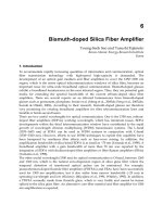


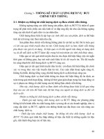

![[Vật Lý Quang Xạ] Kỹ Thuật Laser phần 4 pot](https://media.store123doc.com/images/document/2014_07/14/medium_gwz1405275676.jpg)
![[Viễn Thông] Giáo Trình: Lý Thuyết Thông Tin phần 4 pot](https://media.store123doc.com/images/document/2014_07/14/medium_xpu1405275679.jpg)

![[Điện Tử] Lập Trình Điều Khiển Soft SPS Phần 4 potx](https://media.store123doc.com/images/document/2014_07/25/medium_rau1406287209.jpg)
![[Hóa Học] Ứng Dụng Maltodextrin Phần 4 pot](https://media.store123doc.com/images/document/2014_07/27/medium_bbz1406427654.jpg)