Three-Dimensional Integration and Modeling Part 9 potx
Bạn đang xem bản rút gọn của tài liệu. Xem và tải ngay bản đầy đủ của tài liệu tại đây (5.95 MB, 10 trang )
CAVITY-TYPE INTEGRATED PASSIVES 71
63 64 65 66 67 68
-50
-40
-30
-20
-10
0
dB
Frequency (GHz)
S21 (simulated)
S21 (measured)
S11 (simulated)
S11 (measured)
FIGURE 5.24: Measured and simulated S-parameters of the quasielliptic dual-mode cavity filter with a
rectangular slot for inter coupling between cavities.
upper side): <3 GHz. A study of the dual-mode coupling in each cavity on the basis of the initial
determination of the cavity size resonating at a desired center frequency (66 GHz) is performed
first. Then, the final configuration of the three-pole dual-band filter can be obtained through the
optimization of the intercoupling slot size and offsets via simulation.
All the design parameters for the filters are summarized in Table 5.6. Figure 5.24 shows the
measured per formance of the designed filters with a rectangular slot along with a comparison to the
simulated results. It can be observed that the measured results in the case of a rectangular slot pro-
duce a center frequency of 66.2 GHz with the bandwidth of 1.2 GHz (∼1.81%), and the minimum
insertion loss in the passband around 2.9 dB. The simulation showed a minimum insertion loss of
2.5 dB with a slightly wider 3-dB bandwidth of 1.7 GHz (∼2.58%) around the center frequency
of 65.8 GHz. The center frequency shift is caused by XY shrinkage of ±3%. The two measured
transmission zeros with a rejection better than 34 dB and 37 dB are observed within <1.55 GHz
and <2.1 GHz, respectively, away from the center frequency at the lower band than the passband.
One transmission zero is observed within <1.7 GHz at the higher band than the passband. The
discrepancy of the zero positions and rejection levels between the measurement and the simula-
tion can be attributed to the fabrication tolerances as explained in Section 5.4.1.5. Still, it can be
observed that the behavior of transmission zeros shows a good correlation of measurements and
simulations.
72 THREE-DIMENSIONAL INTEGRATION
L
ext
L
c
port 1 port 2
L
ext
M
12
12
3 4
M
34
M
13
M
24
FIGURE 5.25: Multicoupling diagram for the ver tically stacked multipole dual-mode cavity filter with
a rectangular slot for intercoupling between two cavities.
This type of filter can be used to generate the sharp skirt at the lower side to reject local
oscillator and image signals as well the extra transmission zero in the high skirt that can be utilized
to suppress the harmonic frequencies according to the desired design specifications.
5.4.2.2 Quasi-elliptic Filter with a Cross Slot. The cross slot is applied as an alternative intercoupling
slot between the two vertically stacked cavities. The multipath diagram for the filter and the phase
shifts for the possible signal paths are described in Fig. 5.25 and Table 5.7. Each cavit y supports two
TABLE 5.7: Total phase shifts for three different signal paths in the vertically stacked dual-
mode c avity filter with a cross slot.
PATHS BELOW RESONANCE ABOVE RESONANCE
Port 1-1-2-port 2 −90
◦
+ 90
◦
+ 90
◦
+ 90
◦
−90
◦
=+90
◦
−90
◦
−90
◦
+ 90
◦
−90
◦
−90
◦
=−270
◦
Port 1-port 2 −90
◦
−90
◦
Result Out of phase Out of phase
1-3-4-2 −90
◦
+ 90
◦
+ 90
◦
+ 90−90
=+90
◦
−90
◦
−90
◦
+ 90
◦
−90−90
=−270
◦
1–2 +90
◦
+90
◦
Result In phase In phase
CAVITY-TYPE INTEGRATED PASSIVES 73
60 61 62 63 64 65 66 67
-60
-50
-40
-30
-20
-10
0
dB
Frequency (GHz)
S21 (simulated)
S21 (measured)
S11 (simulated)
S11 (measured)
FIGURE 5.26: Measured and simulated S-parameters of the quasi-elliptic dual-mode cavity filter with
a rectangular slot for inter coupling between cavities.
orthogonal dual modes (1 and 2 in the top cavity, 3 and 4 in the bottom cavity) since the cross-slot
structure excites both degenerate modes in the bottom cavity by allowing the coupling between the
modes that have the same polarizations. The coupling level can be adjusted by varying the size and
position of the cross slots. The couplings of M
12
and M
34
are realized by electrical coupling while
the inter couplings of M
13
and M
24
are realized by magnetic coupling. The total phase shifts of the
four signal paths of the proposed structure prove that they generate one zero above resonance and
one below resonance.
The quasielliptic filters were designed for a sharp selectivity. The simulation achieved the
following specifications: (1) Center frequency: 63 GHz, (2) 3-dB fractional bandwidth: ∼2%, (3)
Insertion loss: <3 dB, and (4) 40 dB rejection bandwidth using two transmission zeros (one on the
lowersideandoneon theupper side):<4 GHz.Thefilter wasfabricatedusingLTCC substratelayers.
Figure 5.26 shows the measured results compared to those of the simulated design. The fabricated
filter exhibits a center frequency of 63.5GHz, an insertion loss of approximately 2.97 dB, a 3-dB
bandwidth of approximately 1.55 GHz (∼2.4%), and >40 dB rejection bandwidth of 3.55 GHz.
74
75
CHAPTER 6
Three-Dimensional Antenna
Architectures
6.1 SOFT-SURFACE STRUCTURES FOR
IMPROVED-EFFICIENCY PATCH ANTENNAS
The radiation performance of patch antennas on large-size substrate can be significantly degraded
by the diffraction of surface waves at the edge of the substrate. Most modern techniques for the
surface-wave suppression are related to periodic structures, such as photonic band-gap (PBG) or
electromagnetic band-gap (EBG) geometries [87–89]. However, those techniques require a con-
siderable area to form a complete band-gap structure. In addition, it is usually difficult for most
printed-circuit technologies to realize such a perforated structure. In this chapter, we present the
novel concept of the “soft surface” to improve the radiation pattern of patch antennas [90]. A single
square ring of shorted quarter-wavelength metal strips is employed to form a soft surface and to sur-
round the patch antenna for the suppression of outward propagating surface waves, thus alleviating
the diffraction at the edge of the substrate. Since only a single ring of metal strips is involved, the
formed“softsurface”structure iscompact andeasilyintegrablewiththree-dimensional(3D)modules.
6.1.1 Investigation of an Ideal Compact Soft Surface Structure
For the sake of simplicity, we consider a probe-fed square patch antenna operating at 15GHz on
a square grounded substrate with thickness H (∼0.025
0,
0
is the free-space wavelength) and a
dielectric constant ε
r
(∼5.4). The patch antenna is surrounded by the ideal compact soft surface that
consists of a square ring of metal strip, that are short-circuited to the ground plane by a metal wall
along the outer edge of the ring, as shown in Fig. 6.1.
The inner length of every side of the soft surface ring (denoted by L
s
) was found to be
approximately one wavelength plus L
p
. The substrate’s size is assumed to be L ×L (2
0
×2
0
),
much larger than the size (L
p
×L
p
< 0.5
g
×0.5
g
) of the square patch. The width of the metal
strip (W
s
) is approximately equal to one quarter of the guided wavelength. The mechanism for the
radiation pattern improvement achieved by the introduction of a compact soft surface structure c an
be understood by considering two factors. First the quarter-wave shorted metal strip serves as an
open circuit for the TM
10
mode (the fundamental operating mode for a patch antenna). Therefore,
it is difficult for the sur face current on the inner edge of the soft surface ring to flow outward
76 THREE-DIMENSIONAL INTEGRATION
FIGURE 6.1: Patch antenna surrounded by an ideal compact soft surface structure consisting of a ring
of metal strip and a ring of shorting wall (I
s
, surface current on the top surface of the soft surface ring,
Z
s
, impedance looking into the shorted metal strip).
(also see Fig. 6.2). As a result, the surface waves can be considerably suppressed outside the soft
surface ring, hence reducing the undesirable diffraction at the edge of the grounded substrate.
Thisexplanationcan beconfirmed bycheckingthe fielddistributionin thesubstrate. Figure6.2
shows the electric field distributions on the top surface of the substrate for the patch antennas with
THREE-DIMENSIONAL ANTENNA ARCHITECTURES 77
FIGURE 6.2: Simulated electric field distributions on the top surface of the substrate for the patch
antennas with (a) and without (b) the soft surface (ε
r
= 5.4).
78 THREE-DIMENSIONAL INTEGRATION
and without the soft surface. We can see that the electric field is indeed contained inside the soft
surface ring. It is estimated that the field magnitude outside the ring is approximately 5 dB lower than
that without the sof t surface. The second factor contributing to the radiation pattern improvement
is the fringing field along the inner edge of the soft surface ring. This fringing field along with the
fringing field at the radiating edges of the patch antenna forms an antenna array in the E-plane. The
formed array acts as a broadside array with minimum radiation in the x-y plane when the distance
between the inner edge of the soft sur face ring and its nearby radiating edge of the patch is roughly
half a wavelength in free space.
6.1.2 Implementation of the Soft-Surface Structure in LTCC
To demonstrate the feasibility of the multilayer LTCC technology on the implementation of the soft
surface, we first simulated a benchmarking prototype that was constr ucted replacing the shortingwall
with a ring of vias. The utilized low temperature cofired ceramic (LTCC) material had a dielectric
constant of 5.4. The whole module consists of a total of 11 LTCC layers (layer thickness=100 m)
and 12 metal layers (layer thickness =10 m). The diameter of each via specified by the fabr ication
process was 100 m, and the distance between the centers of two adjacent vias was 500 m. To
support the vias, a metal pad is required on each metal layer; to simplify the simulation, all pads
on each metal layer are connected by a metal strip with a width of 600 m. Simulation shows that
the width of the pad metal strips has little effect on the performance of the soft surface structure
as long as it is less than the width of the metal strips for the soft surface ring (W
s
). The size of the
LTCC board was 30 mm ×30 mm. The operating frequency was set within the K
u
-band (the design
frequency f
0
=16.5 GHz).
The optimized values for L
s
and W
s
were, respectively, 22.2 mm and 1.4 mm, which led to a
total via number of 200 (51 vias on each side of the square ring). Including the width (300 m) of the
pad metal strip, the total metal strip width for the soft surface ring was found to be 1.7 mm. Since
the substrate was electrically thick at f
0
=16.5 GHz (>0.1
g
), a stacked configuration was adopted
for the patch antenna to improve its input impedance performance. By adjusting the distance
between the stacked square patches, a broadband characteristic for the return loss can be achieved
[91]. For the present case, the upper and lower patches (with the same size 3.4 mm ×3.4 mm) were
respectively printed on the first LTCC layer and the seventh layer from the top, leaving a distance
between the two patches of 6 LTCC layers. The lower patch was connected by a via hole to a 50-
microstrip feed line that was on the bottom surface of the LTCC substrate. The ground plane was
embedded between the second and third LTCC layers from the bottom. The inner conductor of
an SMA (semi-miniaturized type-A) connector was connected to the microstrip feed line while its
outer conductor was soldered on the bottom of the LTCC board to a pair of pads that were shorted
to the ground through via metallization. It has to be noted that the microstrip feed line was printed
on the bottom of the LTCC substrate to avoid its interference with the soft surface ring and to
THREE-DIMENSIONAL ANTENNA ARCHITECTURES 79
12 13 14 15 16 17 18 19 20
-25
-20
-15
-10
-5
0
measured
simulated
Return loss (dB)
Frequency (GHz)
12 13 14 15 16 17 18 19 20
-25
-20
-15
-10
-5
0
measured
simulated
Return loss (dB)
Frequency (GHz)
FIGURE 6.3: Comparison of return loss between simulated and measured results for the stacked-patch
antennas with (a) and without (b) the soft surface implemented on LTCC technology.
alleviate the contribution of its spurious radiation to the radiation pattern at broadside. An identical
stacked-patch antenna on the LTCC substrate without the soft surface ring was also built for
comparison.
The simulated and measured results for the return loss shown in Fig. 6.3 show good agree-
ment. As the impedance performance of the stacked-patch antenna is dominated by the coupling
between the lower and upper patches, the return loss for the stacked-patch antenna seems more
sensitive to the soft surface structure than that for the previous thinner single patch antenna. The
measured return loss is close to −10 dB over the frequency range 15.8–17.4 GHz (about 9% in
bandwidth). The slight discrepancy between the measured and simulated results is mainly due to the
fabrication issues (such as the variation of dielectric constant or/and the deviation of via positions)
and the effect of the transition between the microstrip line and the SMA (SubMiniature version A)
connector.
It is also noted that there is a frequenc y shift of about 0.3 GHz (about 1.5% up). This is
probably caused by the LTCC material that may have a real dielectric constant slightly lower than
the over estimated design value. It is noted that it is normal for practical dielectric substrates to have
a dielectric constant within a ±2% deviation.
The radiation patterns measured in the E- and H-planes show a good agreement with the
simulation with the simulated results in Fig. 6.4 for the frequency of 17 GHz where the maximum
gain of the patch antenna with the sof t surface was observed. It is confirmed that the radiation at
broadside is enhanced and the backside level is reduced. Also the beam width in the E-plane is
significantly reduced by the soft surface, realizing a more directive radiation performance. It is noted
80 THREE-DIMENSIONAL INTEGRATION
E-plane ( =0
o
)
180
o
150
o
120
o
-150
o
-120
o
|E| (dB) -40 -30 -20 -10 0
z
x
-90
o
-60
o
-30
o
30
o
=0
o
60
o
90
o
Measured co-pol.
Simulated co-pol
Measured cross-pol
E-plane ( =0
o
)
180
o
150
o
120
o
-150
o
-120
o
|E| (dB) -40 -30 -20 -10 0
z
x
-90
o
-60
o
-30
o
30
o
=0
o
60
o
90
o
Measured co-pol.
Simulated co-pol.
Measured cross-pol.
(a) E-plane ( =0 )
H-plane ( =90
o
)
180
o
150
o
120
o
-150
o
-120
o
|E| (dB) -40 -30 -20 -10 0
z
y
-90
o
-60
o
-30
o
30
o
=0
o
60
o
90
o
Measured co-pol.
Simulated co-pol
Measured cross-pol.
Simulated cross-pol.
H-plane ( =90
o
)
180
o
150
o
120
o
-150
o
-120
o
|E| (dB) -40 -30 -20 -10 0
z
y
-90
o
-60
o
-30
o
30
o
=0
o
60
o
90
o
Measured co-pol
Simulated co-pol
Measured cross-pol.
Simulated cross-pol.
(b) H-plane ( =90 )
FIGURE 6.4: Compar ison between simulated and measured radiation patterns for the stacked-patch
antennaswith(left) andwithout (right)the soft surfaceimplemented onLTCCtechnology( f
0
=17 GHz).
(a) E-plane ( =0
◦
). (b) H-plane ( =90
◦
).
that the measured cross-polarized component has a higher level and more ripples than the simulation
result. This is because the simulated radiation patterns were plotted in two ideal principal planes,
i.e., =0
◦
and =90
◦
planes. The simulations demonstrated that the maximum cross-polarization
may happen in the plane =45
◦
or =135
◦
. During measurement, a slight deviation from the
ideal planes can cause a considerable variation for the cross-polarized component since the spatial
variation of the cross-polarization is quick and irregular.