A Finite Element Scheme for Shock Capturing Part 2 pptx

Figure
1.
Definition of terms for
a
moving hydraulic jump
Uo
=
velocity at section
0
ho
=
depth at section
0
U1
=
velocity at section
1
hl
=
depth at section
1
Vo
=
Uo
-
V,,
the velocity
at
section
0
relative to the jump

V1
=
U1
-
V,,
relative velocity at section
1
Mass.
Now following an infinitesimal fluid element in our moving coordi-
nate system we know that mass is conserved
so
we have,
where
p,
the fluid density, is a constant here.
Across the element we have
p(Vlhl
-
Vehe)
=
0
Chapter
1
Introduction
where
q
is the relative discharge. Equation
3
may be written in a fixed grid as
v,

[h]
=
[Ula]
(5)
where the symbol
[I
implies the jump in the quantities across the discon-
tinuity,
e.g.,
b]
H
hl
-
ho.
Momentum.
In the same manner we show that momentum is conserved
by:
where
which in
a
fixed coordinate system would be:
V,
[Uh]
=
[u2
h
+
F]
Energy.
Now consider the case of mechanical energy

E
as it passes
through the discontinuity
If we multiply
(8)
by
V,
add this to (10) using
the
relationship for
q
we have:
Chapter
1
Introduction
Now substituting Equation
8
yields
or, finally
so that the shallow-water equations lose energy at the jump, and it is propor-
tional to the depth differential cubed. If the depth is continuous, no
energv
will be lost.
While mathematically an energy gain,
dEldt
>
0,
through the jump is a
possibility, physically it is not. If we restrict ourselves to energy losses
through the jump, there are two possible cases.

a. Case
1:
Vo,
Vl
c
0
implies
ho
9
hl.
The jump progresses
downstream through our fluid
element (Figure 2).
b.
Case
2:
Vo, V1
>
0
implies
ho
c
hl.
The fluid passes
downstream through the jump
(Figure
3).
_____)
Back
I

Front
Figure
2.
Example of Case
1
;
jump
Here we have arbitrarily chosen
passes downstream through
the flow to be from left to right, if
the fluid element
we had chosen the opposite direction
one would simply have horizontal
mirror images of Figures
2
and
3.
A
fluid particle that is about to be swept
into or caught by the jump is considered in "front" of the jump.
A
fluid
element that has passed through the jump is now "behind" it. Therefore, we
mav conclude that the water level is lower in front of the iump than it is
behind the jump.
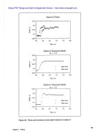
In order to calculate the wave speed, it is convenient to choose
Ul
=
0.
Chapter

1
Introduction
+
++
+
+
Front
I
Back
This is completely arbitrary, and this
form also produces an easy test case
that will be eventually applied to the
numerical model. With
U1
=
0,
then Vl
=
U1
-
Vw
=
-V
the
W'
momentum equation may be written
as:
1
-vw(uo -V,) =?g(ho +hl) (14)
Figure

3.
Example of Case
2;
the fluid
passes downstream through
and now, taking advantage of our
the jump
mass conservation relationship, we
have:
We may substitute for
Uo to yield:
If we consider the speed of the perturbation in front of and behind the shock,
we note that both move toward the shock.
To demonstrate this, we calculate the relative speeds
Vo and V1. These are
the speeds of fluid particles as perceived by an observer moving with the
shock. We have already shown that
Vl
=
-Vw or
The relative speed of an upstream moving perturbation
W1 is
If this value is negative, then a perturbation behind the jump catches the shock,
and from Equation
17
we know dgh, is greater in magnitude than V1, Wl c
0.
In front of the shock the relative particle speed is Vo.
Chapter
1

Introduction
Again we calculate the relative speed of a perturbation, but now in front of
the shock:
Now if
Wo
is positive the shock catches up with the wave perturbation, and
since
Vo
is clearly greater than
dgh,
this is indeed what happens. Therefore
any small perturbations are swept toward, and are engulfed in the shock.
Shock
relations
in
2-D
Previous sections derive the
shock relations in l-D and are
important for understanding behavior
and to produce test problems. Here
we extend these relations to
2-D
(Courant and Friedricks 1948). To
do this, consider the region
52
shown
in Figure
4.
It is divided into
subdomains

Q1
and
SL2
by the shock
shown as boundary
T,,
which is
defined by the coordinate location
X,(t). The right side boundary is
I',
and the left
rl.
The normal
direction is chosen as shown in
Figure
4.
Integration over the
subdomains is performed separately;
and then by letting the width about
Figure
4.
Definition of terms for 2-D
the shock go to zero, we derive the
shock
mass and momentum relationship
across the jump in the direction
n.
Mass conservation.
For constant density we have
Chapter

1
Introduction
which may be expanded as
-
h'
[xdt)
n]
a
+
h, (V,
end
dr
=
0
Jr
where,
Vp
=
the velocity of the left boundary
V,
=
the velocity of the right boundary
xS(t)
=
the velocity of the shock
h-
=
the depth in the limit as the shock is approached
from subdomain
SZ1

h+
=
the depth in the limit as the shock is approached
from subdomain
R2
Taking the limit as
R1
and
R2
shrink in width we have
where,
V'
=
the velocity in the limit as the shock is
approached in subdomain
Q1
V+
=
the velocity in the limit as the shock is
approached in subdomain
n2
For an arbitrary segment
T,
to preserve the equation, the integrand itself
must satisfy the equation, therefore
Chapter
1
Introduction
where
which states that the relative mass flux jump across the shock in the direction

n
should be zero.
Momentum relation.
Again assuming constant density, the balance of
momentum and force may be written as (in the direction of the normal to the
shock)
and taking the limit as
GI
and
Q2
shrink in width results in
Chapter
1
Introduction
which for an arbitrary length
T,
to preserve the equation, the integrand itself
must satisfy the equation, therefore:
where,
Q'
=
V-h-
Q+
=
v+ht
or
which states that the relative momentum flux in the direction
n
is balanced by
the pressure jump across the shock.

Chapter
1 Introduction
2
Numerica Approach
The selection of a numerical scheme is driven by two related difficulties:
numerically modeling highly advective flow and the capturing of shocks. This
chapter discusses the problem with advection schemes generally.
It
then
follows the development of the scheme we will use and discusses the
implications in shock capturing.
Advection Dominated Flow
The
problem
The quality of the numerical solution depends upon the choice of the basis
(or interpolation) function and upon the test function. The basis function
determines how the variable (or solution) is represented and the test function
determines the way in which the differential equation is enforced. Finite ele-
ments are a subset of the weighted residual method. Here one looks at the
solution of a differential equation in a weighted average sense. In the Galerkin
approach the test function is identical to the basis function. This method can
have difficulty with advection-dominated flow. The basic problem is that the
form of the test function (typically an even or symmetric function) cannot
detect the presence of a node-to-node oscillation, since this "spurious solution"
has a spatial derivative which is an odd function (antisymmetric). One
approach to resolve this problem is to use a mixed interpolation where, for the
shallow-water equations, the depth uses a lower order basis than does the
velocity (see,
e.g., Platzman (1978) or Walters and Carey (1983)). Typically,
these are chosen as depth as an elemental constant and velocity as linear, or

depth linear and velocity as a quadratic. This approach effectively decouples
the depth from this node-to-node oscillation but depends upon some additional
artificial viscosity to damp velocity oscillations if the flow is not highly
resolved. Another approach is to modify the test function so that it includes
odd functions as well as even functions so that these modes can be detected
and if weighted properly, eliminated. Any approach in which the test function
differs from the basis function is termed a
Petrov-Galerkin approach.
In
our
case we choose the
Lagrange basis functions to be
CO;
i.e., the functions are
continuous. Let us consider an example to illustrate the problem with the
Calerkin approach and an approach to develop a Petrov-Galerkin test function.
Chapter
2
Numerical Approach
Petrov-Galerkin formulation
First we will illustrate the problem that discrete formulations have with
advection-dominated flow. In this regard the
1-D
linearized inviscid Burgers'
equation may be written
Cl
+
UOC,
=
0

,
over domain
L
(34)
where the subscripts
t
and x represent partial derivatives with respect
to
time
and space, respectively, and
Uo
=
the advection velocity, which here is a constant
C
=
some species concentration
In the discrete representation we shall approximate the solution as
CO
linear
Lagrange basis functions,
here
c(x) is the approximate solution, and the subscript
j
indicates nodal
values and
@j
is the Gaierkin test function at node
j.
Our numerical solution equation, for the steady-state problem (Ct=O) may
be written as the inner product

(@i
,
Uo
$
@j'
(x) Cj)
=
0
,
for
each
i
J
where
Cf(x), d-4)
=
SL
f0
g(x)
dx
and the prime indicates the derivative with respect to x.
On a uniform grid the result of this integration on
a
typical patch is
(Note that finite difference methods using central differences give an identical
result
.)
In order to demonstrate that this solution contains a spurious oscillation,
let's write these nodal values as
Chapter

2
Numerical Approach