A Finite Element Scheme for Shock Capturing Part 4 docx

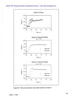
Figure
6.
Time-history of center-line water surface elevation profiles;
9
=
1.0,
Ax
=
0.4
m,
At
=
0.4
sec
Figure
7.
Time-history of center-line water surface elevation profiles;
9
=
1
.O,
Ax
=
0.4
m,
At
=
0.8
sec
Chapter
3

Testing
Figure
8.
Time-history of center-line water surface elevation profiles;
9
=
1.0,
Ax
=
0.4
m,
At
=
1.6
sec
Figure
9.
Time-history
of
center-line water surface elevation profiles;
at
=
1
.O,
Ax
=
0.8
m,
At
=

0.8
sec
Chapter
3
Testing
Figure 10. Time-history of center-line water surface elevation profiles;
at
=
1
.O,
Ax
=
0.8
m,
At
=
1.6 sec
Figure 11. Time-history of center-line water surface elevation profiles;
o+
=
1
.O,
Ax
=
0.8
m, At
=
3.2
sec
Chapter

3
Testing
one moves over time, the center-line profile shock moves upstream. It is apparent that as the
spatial and temporal resolution improve, the shock becomes steeper. The shock is fairly
consistently spread over three or four elements; and so as the element size is reduced, the
resulting shock is steeper. The
x-t
slope of the shock indicates the shock speed. Any bending
would indicate that the speed changed over time, which should not be the case. The upper
elevation is precisely 0.2 m, which is correct. There is no overshoot of the jump, though there
is some undershoot when
C,
is less than
1.
Cs
is the product of the analytic shock speed and
the ratio of time-step length to element length. A
C,
value of
1
indicates that the shock
should move
1
element length in
1
time-step.
Figures 12 and 13 show the error in calculated speed and the relative error in calculated
speed, respectively. These are for
AX
=

0.4, 0.8 and 1.0 m which is reflected in the Grid
Resolution Number defined as
MlAh.
Here
h
is the depth and
Ah
is the analytic depth
difference across the shock, 0.1 m. The error was
as
small as was detectable by the technique
for measurement of speed at
AX
=
0.4 m so there was no need
to
go
to
smaller grid spacing.
Values of
C,
less than
1
appear
to
lag the analytic shock and
Cs
greater than
1
leads the

analytic shock. With the largest
C,
the calculated shock speed is greater than the analytic by
at most 0.0034
mlsec which is only 0.6 percent too fast. As resolution is improved the
solution appears to converge to the analytic speed.
Figures 14-16 and 17-19 are the center-line profile histories for
at
=
1.5 and for
AX
=
0.4
and 0.8 m, respectively. It is apparent that the lower dissipation from this second-order
scheme allows an oscillation which is most notable upstream of the jump for larger values of
C,.
But as
C,
decreases, there is an undershoot in front of the shock. The slope of the
x-t
line along the top of the shock has a significant bend early in the high
Cs
simulations. The
speed is too slow here.
Now consider the associated Figures 20 and 21 for error in calculated shock speed and
relative error in calculated speed. The error is actually worse than for the first-order scheme.
This is due primarily
to
the slow speed early in the simulation; if this is dropped by using only
the last 50 seconds of simulation, the relative error is only 0.6 percent slower than analytic.

Once again, as the resolution improves, the solution converges
to
the proper solution.
Case
2:
Dam Break
This second case is a comparison
to
hydraulic flume results reported in Bell, Elliot, and
Chaudhry (1992).
A
plan view of the flume facility is shown in Figure 22. The flume was
constructed of Plexiglas and simulates a dam break through a horseshoe bend.
This is a more
general comparison than Case
1.
Here the problem is truly 2-D and we now are comparing to
hydraulic flume results, so we must take into consideration the limitations of the shallow-water
equations themselves. Initially, the reservoir has an elevation of 0.1898 m relative to the chan-
nel bed; the channel itself is at a depth (and elevation) of 0.0762 m.
The velocity is zero and
then the dam is removed.
The surge location and height were recorded at several stations, and
our model is compared at three of these, at stations 4, 6, and 8.
Station 4 is 6.00 m from the
dam along the channel center-line in the center of the bend, station 6 is 7.62 m from the dam
near the conclusion of the bend, and station 8 is 9.97 m from the dam in a straight reach. The
model specified parameters are shown in Table
3.
Chapter

3
Testing
Figure
12.
Error in model shock speed with grid refinement for
at
=
1.0
Model Shock Speed Precision
Figure
13.
Relative error
in
model shock speed with grid refinement for
at
=
1
.o
Cs
=
2.191
0
Cs
=
1.095
0
Cs
=
0.548
0.01

2
g
0
W
-0.01
Model Shock Speed Precision
Chapter
3
Testing
"22
Grid
Resolution Number, Delta
X
I
Delta
h
Cl
A
8%
0
I
I I
I
I
0
CI
d
\O
Cs
=

2.191
0
CS
=
1.095
0
Cs
=
0.548
0.02
B
a
V)
3
n
V)
0

*
A
-
4
.
0
8
t:
W
'a
R.
V)

3
n
V)
-0.02
0
CI
d
'0
"
S
2
Grid
Resolution Number, Deita
X
1
Delta
h
+
13
0
A A
-
0
I
1
I
I
I
Figure 14. Time-history of center-line water surface elevation profiles;
9

=
1.5,
Ax
=
0.4
m,
At
=
0.4
sec
Figure 15. Time-history of center-line water surface elevation profiles;
9
=
1.5,
Ax
=
0.4
m,
At
=
0.8
sec
Chapter
3
Testing
Figure
16.
Time-history
of
center-line water surface elevation profiles;

9
=
1.5,
Ax
=
0.4
m,
At
=
1.6
sec
Figure
17.
Time-history of center-line water surface elevation profiles;
3
=
1.5,
&
=
0.8
m, At
=
0.8
sec
Chapter
3
Testing
31
Figure 18. Time-history of center-line water surface elevation profiles;
3

=
1.5,
Ax
=
0.8 m,
At
=
1.6 sec
Figure 19. Time-history of center-line water surface elevation profiles;
9
=
1.5,
Ax
=
0.8 m,
~t
=
3.2
sec
Chapter
3
Testing
Figure 20. Error in model shock speed with grid refinement for
9
=
1.5
Model Shock Speed Precision
Figure 21. Relative error in model shock speed with grid refinement for
at
=

1.5
Chapter
3
Testing
Cs
=
2.191
0
Cs
=
1.095
0
Cs
=
0.548
0.01
2
0
g
W
-0.01
0
2
4
6
8
10
12
Grid
Resolution

Number,
Delta
X
/
Delta
h
0
0
0
A
w
-
V
0
I
I
I
I
I
Chapter
3
Testing