A Finite Element Scheme for Shock Capturing Part 6 potx

where the superscript
n
indicates the time-step and the subscript
j
is the spatial
node location.
We now present the results of this analysis for
a
=
112 and for the temporal
derivative parameter
at
of 1.0 and
1.5.
We shall compare the relative ampli-
tude and relative speed for a single time-step. The parameter for relative speed
is given by
relative
speed
=
tan
where
N
=
elements per wavelength
AAt,
C
=
Courant number
r
-

Ax*
h
=
wave speed, either hl or h2
For
at
=
1,
which is first-order backward difference in time, the relative
amplitude is shown in Figure 29 and the relative wave speed is shown in Fig-
ure 30. This is plotted versus the number of elements per wavelength
N
and
the Courant number
C.
Also
remember that these comparisons apply for either
characteristic
(Al or h2), even for subcritical conditions in which h2 is
negative. In these figures the Courant number varies from
0.5
to 2.0 and the
elements per wavelength from
2
to 10.
The amplitude portrait shows substantial damping for larger
C
and for the
shorter wavelengths (or alternatively the poorer resolution). The large damp-
ing at a wavelength of

2Ax
is important, as this is the mechanism that provides
the energy dissipation to capture shocks. Now consider the phase portrait, or
in this case the relative speed portrait. Over the conditions shown, the numeri-
cal speed is less than
the
analytic speed throughout. For larger
C
the relative
speed is somewhat lower (worse). For
N
=
2 the speed is
0,
so that undamped
oscillation could remain at steady state.
Chapter
3
Testing
Figure
29.
Relative amplitude versus
C
and resolution for
at
=
1.0 and
a
=
0.5

Figure 30. Relative speed versus
C
and resolution for
at
=
1.0 and
a
=
0.5
Chapter
3
Testing
In comparison to the results we have shown in Figures 6-11 for Case
1,
analytic shock case, we must remember that C, is the Courant number based
on shock speed, whereas
C
is based on the perturbation wave speed. If we
consider a wave moving upstream just behind the shock, since short wave-
lengths move
t~o slowly, the disturbance of the shock produces waves of these
length which fall behind the shock rather than remaining within.
As
the time-
step is reduced (C, gets smaller) the relative speed is better for the moderate
wavelengths and so the
shock front becomes sharper.
At a point near the shock front we note that generally we get a sharp front
with no undershoot until we reach the smallest time-step. Again if we are
within the shock at a depth where there is an upstream propagating wave

(subcritical), is there a Courant number C that has a relative speed greater than
analytic. This would be the only way in which an undershoot could appear.
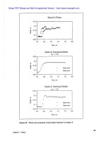
Figure
31
extends the relative wave speed portrait below
C
=
0.5. From this
figure it is apparent for small values of C that the numerical wave speed is
greater than analytic so that it is possible to develop an undershoot in front of
the jump.
For
at
=
1.5 we have a second-order temporal derivative which has relative
amplitude and relative speed portraits shown in Figures 32 and 33, respec-
tively.
The degree of damping is much less than for the first-order case. The
relative speed is better but not so dramatic as the improvement in amplitude.
An
interesting point is that the relative speed for
N
=
2
is nonzero for lower C
values. This implies that a spurious mode should not reside in the grid at
steady state. In Figure
34,
we show the relative speed portrait extended below
C values of 0.5.

As
with
q
=
1,
for very low C the numerical relative speed
is greater than the analytic. Therefore, we would expect to have an undershoot
for small time-steps. It should become more pronounced and longer as the
time-step is reduced further. Since we generally have
a
relative speed lower
than analytic, we expect an overshoot behind the jump which becomes longer
as the time-step is increased. Referring to Figures 14-19 of case 1, this is
precisely what we note. Also, for smaller time-steps there is some undershoot
as well. These same features are notable in the second test case, the dam
break test case.
For the sake of completeness the relative amplitude and speed portraits are
included for
a
=
0 and 0.25 at
at
of 1.0 and 1.5 in Figures 35-42. The condi-
tion
a
=
0 is, in fact, the Galerkin case since the Petrov-Galerkin contribution
is included through
a.
The Galerkin approach is shown to contain a steady-

state spurious mode due to the speed of zero for
N
=
2. Furthermore, this
mode is undamped. The case of
a
=
0.25 shows that the relative speed
portraits change very little from
a
=
0.5 but the amplitude damping is
improved.
The obvious conclusions that can be drawn from this discussion is that for
an unsteady run either use
at
=
1.5 or take smaller time-steps with
at
=
1.0.
An
improvement in spatial resolution dramatically improves the solution.
Chapter
3
Testing
Relative Speed
0
-
Elements per Wavelength

10
Figure
31.
Relative speed versus
C
and resolution for
at
=
1.0 and
a
=
0.5, for
small values of
C
Relative Amplitude
0.
Elements per Wavelength
Figure
32.
Relative amplitude versus
C
and resolution for
at
=
1.5 and
a
=
0.5
Chapter
3

Testing
Relative Speed
0
.
Elements per Wavelength
Figure
33.
Relative speed versus
C
and resolution for
at
=
1.5 and
a
=
0.5
Relative Speed
0
.
Elements per Wavelength
10
Figure
34.
Relative speed versus
C
and resolution for
at
=
1.5 and
a

=
0.5, for
small values of
C
Chapter
3
Testing
Figure
35.
Relative amplitude versus
C
and resolution for
at
=
1.0
and
a
=
0
Elements per Wavelength
Figure
36.
Relative speed versus
C
and resolution for
at
=
1.0
and
a

=
0
Chapter
3
Testing
Relative Amplitude
o.
Elements per Wavelength
Figure
37.
Relative amplitude versus
C
and resolution for
at
=
1.0 and
a
=
0.25
Elements per Wavelength
Figure
38.
Relative speed versus
C
and resolution for
at
=
1
.O and
a

=
0.25
Chapter
3
Testing
Relative Amplitude
o.
Elements per Wavelen
Figure
39.
Relative amplitude versus
C
and resolution for
at
=
1.5
and
a
=
0
Relative Speed
0.
Elements per Wavelength
Figure
40.
Relative speed versus
C
and resolution for
at
=

1.5
and
a
=
0
Chapter
3
Testing
Relative Amplitude
Elements per Wavelength
Figure 41. Relative amplitude versus
C
and resolution for
at
=
1.5 and
a
=
0.25
Figure 42. Relative speed versus
C
and resolution for
at
=
1.5
and
a
=
0.25
Chapter

3
Testing
4
Conclusions
In this report an algorithm is developed to address the numerical difficulties
in modeling surges and jumps in a computational hydraulics model. The
model itself is a finite element computer code representing the 2-D shallow
water equations.
The technique developed to address the case of advection-dominated flow is
a dissipative technique that serves well for the capturing of shocks. The
dissipative mechanism is large for short wavelengths, thus enforcing energy
loss through the hydraulic jump, unlike a nondissipative technique used on
C"
representation of depth, which will implicitly enforce energy conservation,
dictated by the shallow-water equations, through a
2A.x
oscillation.
The test cases demonstrate that the resulting model converges to the correct
heights and shock speeds with increasing resolution. Furthermore, general 2-D
cases of lateral transition in supercritical flow showed the model to compare
quite well in reproducing the oblique shock pattern.
The trigger mechanism, based upon energy variation, appears to detect the
jump quite well. The Petrov-Galerkin technique shown is an intuitive method
relying upon characteristic speeds and directions and produces a 2-D model
which is adequate to address hydraulic problems involving jumps and oblique
shocks.
The resulting improved numerical model will have application in
supercriti-
cal as well as subcritical channels, and transitions between regimes. The
model can determine the water surface heights along channels and around

bridges, confluences, and bends for a variety of numerically challenging events
such as hydraulic jumps, hydropower surges, and dam breaks. Furthermore,
the basic concepts developed are applicable to models of aerodynamic flow
fields, providing enhanced stability
in
calculation of shocks on engine or heli-
copter rotors, for example, as well as on high-speed aircraft.
Chapter 4
Discussion