A HEAT TRANSFER TEXTBOOK - THIRD EDITION Episode 1 Part 4 potx

64 Heat conduction, thermal resistance, and the overall heat transfer coefficient §2.3
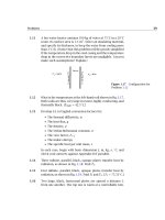
Figure 2.9 The one-dimensional flow of
current.
proportional to the gradient of its mass concentration, m
1
. Thus

j
1
=−ρD
12
∇m
1
(2.19)
where the constant D
12
is the binary diffusion coefficient.
Example 2.3
Air fills a thin tube 1 m in length. There is a small water leak at one
end where the water vapor concentration builds to a mass fraction of
0.01. A desiccator maintains the concentration at zero on the other
side. What is the steady flux of water from one side to the other if
D
12
is 2.84 ×10
−5
m
2
/s and ρ = 1.18 kg/m
3
?

Solution.




j
water vapor



= 1.18
kg
m
3

2.84 ×10
−5
m
2
s


0.01 kg H
2
O/kg mixture
1m

= 3.35 ×10
−7
kg

m
2
·s
Contact resistance
One place in which the usefulness of the electrical resistance analogy be-
comes immediately apparent is at the interface of two conducting media.
No two solid surfaces will ever form perfect thermal contact when they
are pressed together. Since some roughness is always present, a typical
plane of contact will always include tiny air gaps as shown in Fig. 2.10
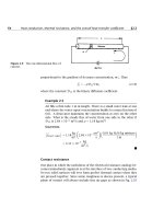
§2.3 Thermal resistance and the electrical analogy 65
Figure 2.10 Heat transfer through the contact plane between
two solid surfaces.
(which is drawn with a highly exaggerated vertical scale). Heat transfer
follows two paths through such an interface. Conduction through points
of solid-to-solid contact is very effective, but conduction through the gas-
filled interstices, which have low thermal conductivity, can be very poor.
Thermal radiation across the gaps is also inefficient.
We treat the contact surface by placing an interfacial conductance, h
c
,
in series with the conducting materials on either side. The coefficient h
c
is similar to a heat transfer coefficient and has the same units, W/m
2
K. If
∆T is the temperature difference across an interface of area A, then Q =
Ah
c
∆T . It follows that Q = ∆T/R
t

for a contact resistance R
t
= 1/(h
c
A)
in K/W.
The interfacial conductance, h
c
, depends on the following factors:
• The surface finish and cleanliness of the contacting solids.
• The materials that are in contact.
• The pressure with which the surfaces are forced together. This may
vary over the surface, for example, in the vicinity of a bolt.
• The substance (or lack of it) in the interstitial spaces. Conductive
shims or fillers can raise the interfacial conductance.
• The temperature at the contact plane.
The influence of contact pressure is usually a modest one up to around
10 atm in most metals. Beyond that, increasing plastic deformation of
66 Heat conduction, thermal resistance, and the overall heat transfer coefficient §2.3
Table 2.1 Some typical interfacial conductances for normal
surface finishes and moderate contact pressures (about 1 to 10
atm). Air gaps not evacuated unless so indicated.
Situation h
c
(W/m
2
K)
Iron/aluminum (70 atm pressure) 45, 000
Copper/copper 10, 000 − 25, 000
Aluminum/aluminum 2, 200 − 12, 000

Graphite/metals 3, 000 − 6, 000
Ceramic/metals 1, 500 − 8, 500
Stainless steel/stainless steel 2, 000 − 3, 700
Ceramic/ceramic 500 −3, 000
Stainless steel/stainless steel
(evacuated interstices)
200 −1, 100
Aluminum/aluminum (low pressure
and evacuated interstices)
100 −400
the local contact points causes h
c
to increase more dramatically at high
pressure. Table 2.1 gives typical values of contact resistances which bear
out most of the preceding points. These values have been adapted from
[2.1, Chpt. 3] and [2.2]. Theories of contact resistance are discussed in
[2.3] and [2.4].
Example 2.4
Heat flows through two stainless steel slabs (k = 18 W/m·K) that are
pressed together. The slab area is A = 1m
2
. How thick must the
slabs be for contact resistance to be negligible?
Solution. With reference to Fig. 2.11, we can write
R
total
=
L
kA
+

1
h
c
A
+
L
kA
=
1
A

L
18
+
1
h
c
+
L
18

Since h
c
is about 3,000 W/m
2
K,
2L
18
must be 
1

3000
= 0.00033
Thus, L must be large compared to 18(0.00033)/2 = 0.003 m if contact
resistance is to be ignored. If L = 3 cm, the error is about 10%.
§2.3 Thermal resistance and the electrical analogy 67
Figure 2.11 Conduction through two
unit-area slabs with a contact resistance.
Resistances for cylinders and for convection
As we continue developing our method of solving one-dimensional heat
conduction problems, we find that other avenues of heat flow may also be
expressed as thermal resistances, and introduced into the solutions that
we obtain. We also find that, once the heat conduction equation has been
solved, the results themselves may be used as new thermal resistances.
Example 2.5 Radial Heat Conduction in a Tube
Find the temperature distribution and the heat flux for the long hollow
cylinder shown in Fig. 2.12.
Solution.
Step 1. T = T(r)
Step 2.
1
r
∂
∂r

r
∂T
∂r

+
1

r
2
∂
2
T
∂φ
2
+
∂
2
T
∂z
2
  
=0, since T ≠ T (φ, z)
+
˙
q
k

=0
=
1
α
∂T
∂T

 
=0, since steady
Step 3. Integrate once: r

∂T
∂r
= C
1
; integrate again: T = C
1
ln r +C
2
Step 4. T(r = r
i
) = T
i
and T(r = r
o
) = T
o
68 Heat conduction, thermal resistance, and the overall heat transfer coefficient §2.3
Figure 2.12 Heat transfer through a cylinder with a fixed wall
temperature (Example 2.5).
Step 5.
T
i
= C
1
ln r
i
+C
2
T
o

= C
1
ln r
o
+C
2
⇒









C
1
=
T
i
−T
o
ln(r
i
/r
o
)
=−
∆T

ln(r
o
/r
i
)
C
2
= T
i
+
∆T
ln(r
o
/r
i
)
ln r
i
Step 6. T = T
i
−
∆T
ln(r
o
/r
i
)
(ln r −ln r
i
) or

T − T
i
T
o
−T
i
=
ln(r /r
i
)
ln(r
o
/r
i
)
(2.20)
Step 7. The solution is plotted in Fig. 2.12. We see that the temper-
ature profile is logarithmic and that it satisfies both boundary
conditions. Furthermore, it is instructive to see what happens
when the wall of the cylinder is very thin, or when r
i
/r
o
is close
to 1. In this case:
ln(r /r
i
) 
r
r

i
−1 =
r − r
i
r
i
§2.3 Thermal resistance and the electrical analogy 69
and
ln(r
o
/r
i
) 
r
o
−r
i
r
i
Thus eqn. (2.20) becomes
T − T
i
T
o
−T
i
=
r − r
i
r

o
−r
i
which is a simple linear profile. This is the same solution that
we would get in a plane wall.
Step 8. At any station, r :
q
radial
=−k
∂T
∂r
=+
l∆T
ln(r
o
/r
i
)
1
r
So the heat flux falls off inversely with radius. That is reason-
able, since the same heat flow must pass through an increasingly
large surface as the radius increases. Let us see if this is the case
for a cylinder of length l:
Q(W) =
(
2πrl
)
q =
2πkl∆T

ln(r
o
/r
i
)
≠ f(r) (2.21)
Finally, we again recognize Ohm’s law in this result and write
the thermal resistance for a cylinder:
R
t
cyl
=
ln(r
o
/r
i
)
2πlk

K
W

(2.22)
This can be compared with the resistance of a plane wall:
R
t
wall
=
L
kA


K
W

Both resistances are inversely proportional to k, but each re-
flects a different geometry.
In the preceding examples, the boundary conditions were all the same
—a temperature specified at an outer edge. Next let us suppose that the
temperature is specified in the environment away from a body, with a
heat transfer coefficient between the environment and the body.
70 Heat conduction, thermal resistance, and the overall heat transfer coefficient §2.3
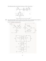
Figure 2.13 Heat transfer through a cylinder with a convective
boundary condition (Example 2.6).
Example 2.6 A Convective Boundary Condition
A convective heat transfer coefficient around the outside of the cylin-
der in Example 2.5 provides thermal resistance between the cylinder
and an environment at T = T
∞
, as shown in Fig. 2.13. Find the tem-
perature distribution and heat flux in this case.
Solution.
Step 1 through 3. These are the same as in Example 2.5.
Step 4. The first boundary condition is T(r = r
i
) = T
i
. The second
boundary condition must be expressed as an energy balance at
the outer wall (recall Section 1.3).
q

convection
= q
conduction
at the wall
or
h(T − T
∞
)
r =r
o
=−k
∂T
∂r




r =r
o
Step 5. From the first boundary condition we obtain T
i
= C
1
ln r
i
+
C
2
. It is easy to make mistakes when we substitute the general
solution into the second boundary condition, so we will do it in

§2.3 Thermal resistance and the electrical analogy 71
detail:
h

(C
1
ln r +C
2
) − T
∞

r =r
o
=−k

∂
∂r
(C
1
ln r +C
2
)

r =r
o
(2.23)
A common error is to substitute T = T
o
on the lefthand side
instead of substituting the entire general solution. That will do

no good, because T
o
is not an accessible piece of information.
Equation (2.23) reduces to:
h(T
∞
−C
1
ln r
o
−C
2
) =
kC
1
r
o
When we combine this with the result of the first boundary con-
dition to eliminate C
2
:
C
1
=−
T
i
−T
∞
k


(hr
o
) + ln(r
o
/r
i
)
=
T
∞
−T
i
1/Bi + ln(r
o
/r
i
)
Then
C
2
= T
i
−
T
∞
−T
i
1/Bi + ln(r
o
/r

i
)
ln r
i
Step 6.
T =
T
∞
−T
i
1/Bi + ln(r
o
/r
i
)
ln(r /r
i
) + T
i
This can be rearranged in fully dimensionless form:
T − T
i
T
∞
−T
i
=
ln(r /r
i
)

1/Bi + ln(r
o
/r
i
)
(2.24)
Step 7. Let us fix a value of r
o
/r
i
—say, 2—and plot eqn. (2.24) for
several values of the Biot number. The results are included
in Fig. 2.13. Some very important things show up in this plot.
When Bi  1, the solution reduces to the solution given in Ex-
ample 2.5. It is as though the convective resistance to heat flow
were not there. That is exactly what we anticipated in Section 1.3
for large Bi. When Bi  1, the opposite is true: (T −T
i
)

(T
∞
−T
i
)
72 Heat conduction, thermal resistance, and the overall heat transfer coefficient §2.3
Figure 2.14 Thermal circuit with two
resistances.
remains on the order of Bi, and internal conduction can be ne-
glected. How big is big and how small is small? We do not

really have to specify exactly. But in this case Bi < 0.1 signals
constancy of temperature inside the cylinder with about ±3%.
Bi > 20 means that we can neglect convection with about 5%
error.
Step 8. q
radial
=−k
∂T
∂r
= k
T
i
−T
∞
1/Bi + ln(r
o
/r
i
)
1
r
This can be written in terms of Q (W) = q
radial
(2πrl) for a cylin-
der of length l:
Q =
T
i
−T
∞

1
h 2πr
o
l
+
ln(r
o
/r
i
)
2πkl
=
T
i
−T
∞
R
t
conv
+R
t
cond
(2.25)
Equation (2.25) is once again analogous to Ohm’s law. But this time
the denominator is the sum of two thermal resistances, as would be
the case in a series circuit. We accordingly present the analogous
electrical circuit in Fig. 2.14.
The presence of convection on the outside surface of the cylinder
causes a new thermal resistance of the form
R

t
conv
=
1
hA
(2.26)
where A is the surface area over which convection occurs.
Example 2.7 Critical Radius of Insulation
An interesting consequence of the preceding result can be brought out
with a specific example. Suppose that we insulate a 0.5 cm O.D. copper
steam line with 85% magnesia to prevent the steam from condensing
§2.3 Thermal resistance and the electrical analogy 73
Figure 2.15 Thermal circuit for an
insulated tube.
too rapidly. The steam is under pressure and stays at 150
◦
C. The
copper is thin and highly conductive—obviously a tiny resistance in
series with the convective and insulation resistances, as we see in
Fig. 2.15. The condensation of steam inside the tube also offers very
little resistance.
3
But on the outside, a heat transfer coefficient of h
=20W/m
2
K offers fairly high resistance. It turns out that insulation
can actually improve heat transfer in this case.
The two significant resistances, for a cylinder of unit length (l =
1 m), are
R

t
cond
=
ln(r
o
/r
i
)
2πkl
=
ln(r
o
/r
i
)
2π(0.074)
K/W
R
t
conv
=
1
2πr
o
h
=
1
2π(20)r
o
K/W

Figure 2.16 is a plot of these resistances and their sum. A very inter-
esting thing occurs here. R
t
conv
falls off rapidly when r
o
is increased,
because the outside area is increasing. Accordingly, the total resis-
tance passes through a minimum in this case. Will it always do so?
To find out, we differentiate eqn. (2.25), again setting l = 1m:
dQ
dr
o
=
(T
i
−T
∞
)

1
2πr
o
h
+
ln(r
o
/r
i
)

2πk

2

−
1
2πr
2
o
h
+
1
2πkr
o

= 0
When we solve this for the value of r
o
= r
crit
at which Q is maximum
and the total resistance is minimum, we obtain
Bi = 1 =
hr
crit
k
(2.27)
In the present example, adding insulation will increase heat loss in-
3
Condensation heat transfer is discussed in Chapter 8. It turns out that h is generally

enormous during condensation so that R
t
condensation
is tiny.
74 Heat conduction, thermal resistance, and the overall heat transfer coefficient §2.3
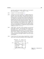
4
2
2.52.01.51.0
2.32
Radius ratio, r
o
/r
i
Thermal resistance, R
t
(K/W)
0
R
t
cond
R
t
cond
+ R
t
conv
r
crit
= 1.48 r
i

R
t
conv
Figure 2.16 The critical radius of insulation (Example 2.7),
written for a cylinder of unit length (l = 1 m).
stead of reducing it, until r
crit
= k

h = 0.0037 m or r
crit
/r
i
= 1.48.
Indeed, insulation will not even start to do any good until r
o
/r
i
= 2.32
or r
o
= 0.0058 m. We call r
crit
the critical radius of insulation.
There is an interesting catch here. For most cylinders, r
crit
< r
i
and
the critical radius idiosyncrasy is of no concern. If our steam line had a 1

cm outside diameter, the critical radius difficulty would not have arisen.
When cooling smaller diameter cylinders, such as electrical wiring, the
critical radius must be considered, but one need not worry about it in
the design of most large process equipment.
Resistance for thermal radiation
We saw in Chapter 1 that the net radiation exchanged by two objects is
given by eqn. (1.34):
Q
net
= A
1
F
1–2
σ

T
4
1
−T
4
2

(1.34)
When T
1
and T
2
are close, we can approximate this equation using a
radiation heat transfer coefficient, h
rad

. Specifically, suppose that the
temperature difference, ∆T = T
1
− T
2
, is small compared to the mean
temperature, T
m
= (T
1
+ T
2
)

2. Then we can make the following expan-
§2.3 Thermal resistance and the electrical analogy 75
sion and approximation:
Q
net
= A
1
F
1–2
σ

T
4
1
−T
4

2

= A
1
F
1–2
σ(T
2
1
+T
2
2
)(T
2
1
−T
2
2
)
= A
1
F
1–2
σ(T
2
1
+T
2
2
)


 
= 2T
2
m
+(∆T)
2
/2
(T
1
+T
2
)

 
=2T
m
(T
1
−T
2
)

 
=∆T
 A
1

4σT
3

m
F
1–2


 
≡h
rad
∆T (2.28)
where the last step assumes that (∆T)
2
/2  2T
2
m
or (∆T/T
m
)
2
/4  1.
Thus, we have identified the radiation heat transfer coefficient
Q
net
= A
1
h
rad
∆T
h
rad
= 4σT

3
m
F
1–2



for

∆T

T
m

2

4  1 (2.29)
This leads us immediately to the introduction of a radiation thermal re-
sistance, analogous to that for convection:
R
t
rad
=
1
A
1
h
rad
(2.30)
For the special case of a small object (1) in a much larger environment

(2), the transfer factor is given by eqn. (1.35)asF
1–2
= ε
1
, so that
h
rad
= 4σT
3
m
ε
1
(2.31)
If the small object is black, its emittance is ε
1
= 1 and h
rad
is maximized.
For a black object radiating near room temperature, say T
m
= 300 K,
h
rad
= 4(5.67 × 10
−8
)(300)
3
 6 W/m
2
K

This value is of approximately the same size as
h for natural convection
into a gas at such temperatures. Thus, the heat transfer by thermal radi-
ation and natural convection into gases are similar. Both effects must be
taken into account. In forced convection in gases, on the other hand,
h
might well be larger than h
rad
by an order of magnitude or more, so that
thermal radiation can be neglected.
76 Heat conduction, thermal resistance, and the overall heat transfer coefficient §2.3
Example 2.8
An electrical resistor dissipating 0.1 W has been mounted well away
from other components in an electronical cabinet. It is cylindrical
with a 3.6 mm O.D. and a length of 10 mm. If the air in the cabinet
is at 35
◦
C and at rest, and the resistor has h = 13 W/m
2
K for natural
convection and ε = 0.9, what is the resistor’s temperature? Assume
that the electrical leads are configured so that little heat is conducted
into them.
Solution. The resistor may be treated as a small object in a large
isothermal environment. To compute h
rad
, let us estimate the resis-
tor’s temperature as 50
◦
C. Then

T
m
= (35 + 50)/2  43
◦
C = 316 K
so
h
rad
= 4σT
3
m
ε = 4(5.67 × 10
−8
)(316)
3
(0.9) = 6.44 W/m
2
K
Heat is lost by natural convection and thermal radiation acting in
parallel. To find the equivalent thermal resistance, we combine the
two parallel resistances as follows:
1
R
t
equiv
=
1
R
t
rad

+
1
R
t
conv
= Ah
rad
+Ah = A

h
rad
+h

Thus,
R
equiv
=
1
A

h
rad
+h

A calculation shows A = 133 mm
2
= 1.33 × 10
−4
m
2

for the resistor
surface. Thus, the equivalent thermal resistance is
R
t
equiv
=
1
(1.33 × 10
−4
)(13 + 6.44)
= 386.8 K/W
Since
Q =
T
resistor
−T
air
R
t
equiv
We find
T
resistor
= T
air
+Q · R
t
equiv
= 35 + (0.1)(386.8) = 73.68
◦

C
§2.3 Thermal resistance and the electrical analogy 77
T
resistor
Q
conv
Q
rad
Q
conv
Q
rad
T
resistor
T
air
R
t
conv
=
1
–
hA
R
t
rad
=
1
h
rad

A
Figure 2.17 An electrical resistor cooled
by convection and radiation.
We guessed a resistor temperature of 50
◦
C in finding h
rad
. Re-
computing with this higher temperature, we have T
m
= 327 K and
h
rad
= 7.17 W/m
2
K. If we repeat the rest of the calculation, we get a
new value T
resistor
= 72.3
◦
C. Further iteration is not needed.
Since the use of h
rad
is an approximation, we should check its
applicability:
1
4

∆T
T

m

2
=
1
4

72.3 − 35.0
327

2
= 0.00325  1
In this case, the approximation is a very good one.
Example 2.9
Suppose that power to the resistor in Example 2.8 is turned off. How
long does it take to cool? The resistor has k  10 W/m·K, ρ 
2000 kg/m
3
, and c
p
 700 J/kg·K.
Solution. The lumped capacity model, eqn. (1.22), may be appli-
cable. To find out, we check the resistor’s Biot number, noting that
the parallel convection and radiation processes have an effective heat
78 Heat conduction, thermal resistance, and the overall heat transfer coefficient §2.4
transfer coefficient h
eff
= h + h
rad
= 18.44 W/m

2
K. Then,
Bi =
h
eff
r
o
k
=
(18.44)(0.0036/2)
10
= 0.0033  1
so eqn. (1.22) can be used to describe the cooling process. The time
constant is
T =
ρc
p
V
h
eff
A
=
(2000)(700)π(0.010)(0.0036)
2
/4
(18.44)(1.33 × 10
−4
)
= 58.1s
From eqn. (1.22) with T

0
= 72.3
◦
C
T
resistor
= 35.0 + (72.3 − 35.0)e
−t/58.1 ◦
C
Ninety-five percent of the total temperature drop has occured when
t = 3T = 174 s.
2.4 Overall heat transfer coefficient, U
Definition
We often want to transfer heat through composite resistances, as shown
in Fig. 2.18. It is very convenient to have a number, U, that works like
this
4
:
Q = UA∆T
(2.32)
This number, called the overall heat transfer coefficient, is defined largely
by the system, and in many cases it proves to be insensitive to the oper-
ating conditions of the system. In Example 2.6, for example, we can use
the value Q given by eqn. (2.25)toget
U =
Q(W)

2πr
o
l(m

2
)

∆T(
◦
C)
=
1
1
h
+
r
o
ln(r
o
/r
i
)
k
(W/m
2
K) (2.33)
We have based U on the outside area, A
o
= 2πr
o
l, in this case. We might
instead have based it on inside area, A
i
= 2πr

i
l, and obtained
U =
1
r
i
hr
o
+
r
i
ln(r
o
/r
i
)
k
(2.34)
4
This U must not be confused with internal energy. The two terms should always
be distinct in context.
§2.4 Overall heat transfer coefficient, U 79
Figure 2.18 A thermal circuit with many
resistances.
It is therefore important to remember which area an overall heat trans-
fer coefficient is based on. It is particularly important that A and U be
consistent when we write Q = UA∆T .
Example 2.10
Estimate the overall heat transfer coefficient for the tea kettle shown
in Fig. 2.19. Note that the flame convects heat to the thin aluminum.

The heat is then conducted through the aluminum and finally con-
vected by boiling into the water.
Solution. We need not worry about deciding which area to base A
on because the area normal to the heat flux vector does not change.
We simply write the heat flow
Q =
∆T

R
t
=
T
flame
−T
boiling water
1
hA
+
L
k
Al
A
+
1
h
b
A
and apply the definition of U
U =
Q

A∆T
=
1
1
h
+
L
k
Al
+
1
h
b
Let us see what typical numbers would look like in this example: h
might be around 200 W/m
2
K; L

k
Al
might be 0.001 m/(160 W/m·K)
or 1/160,000 W/m
2
K; and h
b
is quite large— perhaps about 5000
W/m
2
K. Thus:
U 

1
1
200
+
1
160, 000
+
1
5000
= 192.1 W/m
2
K
80 Heat conduction, thermal resistance, and the overall heat transfer coefficient §2.4
Figure 2.19 Heat transfer through the bottom of a tea kettle.
It is clear that the first resistance is dominant, as is shown in Fig. 2.19.
Notice that in such cases
UA → 1/R
t
dominant
(2.35)
where A is any area (inside or outside) in the thermal circuit.
Experiment 2.1
Boil water in a paper cup over an open flame and explain why you can
do so. [Recall eqn. (2.35) and see Problem 2.12.]
Example 2.11
A wall consists of alternating layers of pine and sawdust, as shown
in Fig. 2.20). The sheathes on the outside have negligible resistance
and
h is known on the sides. Compute Q and U for the wall.
Solution. So long as the wood and the sawdust do not differ dramat-

ically from one another in thermal conductivity, we can approximate
the wall as a parallel resistance circuit, as shown in the figure.
5
The
5
For this approximation to be exact, the resistances must be equal. If they differ
radically, the problem must be treated as two-dimensional.
§2.4 Overall heat transfer coefficient, U 81
Figure 2.20 Heat transfer through a composite wall.
total thermal resistance of the circuit is
R
t
total
= R
t
conv
+
1

1
R
t
pine
+
1
R
t
sawdust

+R

t
conv
Thus
Q =
∆T
R
t
total
=
T
∞
1
−T
∞
r
1
hA
+
1

k
p
A
p
L
+
k
s
A
s

L

+
1
hA
and
U =
Q
A∆T
=
1
2
h
+
1

k
p
L
A
p
A
+
k
s
L
A
s
A


The approach illustrated in this example is very widely used in calcu-
lating U values for the walls and roofs houses and buildings. The thermal
resistances of each structural element — insulation, studs, siding, doors,
windows, etc. — are combined to calculate U or R
t
total
, which is then used
together with weather data to estimate heating and cooling loads [2.5].
82 Heat conduction, thermal resistance, and the overall heat transfer coefficient §2.4
Table 2.2 Typical ranges or magnitudes of U
Heat Exchange Configuration U (W/m
2
K)
Walls and roofs dwellings with a 24 km/h
outdoor wind:
• Insulated roofs 0.3−2
• Finished masonry walls 0.5−6
• Frame walls 0.3−5
• Uninsulated roofs 1.2−4
Single-pane windows ∼ 6
†
Air to heavy tars and oils As low as 45
Air to low-viscosity liquids As high as 600
Air to various gases 60−550
Steam or water to oil 60−340
Liquids in coils immersed in liquids 110−2, 000
Feedwater heaters 110−8, 500
Air condensers 350−780
Steam-jacketed, agitated vessels 500−1, 900
Shell-and-tube ammonia condensers 800−1, 400

Steam condensers with 25
◦
C water 1, 500−5, 000
Condensing steam to high-pressure
boiling water
1, 500−10, 000
†
Main heat loss is by infiltration.
Typical values of U
In a fairly general use of the word, a heat exchanger is anything that
lies between two fluid masses at different temperatures. In this sense a
heat exchanger might be designed either to impede or to enhance heat
exchange. Consider some typical values of U shown in Table 2.2, which
were assembled from a variety of technical sources. If the exchanger
is intended to improve heat exchange, U will generally be much greater
than 40 W/m
2
K. If it is intended to impede heat flow, it will be less than
10 W/m
2
K—anywhere down to almost perfect insulation. You should
have some numerical concept of relative values of U, so we recommend
that you scrutinize the numbers in Table 2.2. Some things worth bearing
in mind are:
• The fluids with low thermal conductivities, such as tars, oils, or any
of the gases, usually yield low values of
h. When such fluid flows
on one side of an exchanger, U will generally be pulled down.
§2.4 Overall heat transfer coefficient, U 83
• Condensing and boiling are very effective heat transfer processes.

They greatly improve U but they cannot override one very small
value of
h on the other side of the exchange. (Recall Example 2.10.)
In fact:
• For a high U, all resistances in the exchanger must be low.
• The highly conducting liquids, such as water and liquid metals, give
high values of
h and U.
Fouling resistance
Figure 2.21 shows one of the simplest forms of a heat exchanger—a pipe.
The inside is new and clean on the left, but on the right it has built up a
layer of scale. In conventional freshwater preheaters, for example, this
scale is typically MgSO
4
(magnesium sulfate) or CaSO
4
(calcium sulfate)
which precipitates onto the pipe wall after a time. To account for the re-
sistance offered by these buildups, we must include an additional, highly
empirical resistance when we calculate U. Thus, for the pipe shown in
Fig. 2.21,
U



older pipe
based on A
i
=
1

1
h
i
+
r
i
ln(r
o
/r
p
)
k
insul
+
r
i
ln(r
p
/r
i
)
k
pipe
+
r
i
r
o
h
o

+R
f
Figure 2.21 The fouling of a pipe.
84 Heat conduction, thermal resistance, and the overall heat transfer coefficient §2.4
Table 2.3 Some typical fouling resistances for a unit area.
Fluid and Situation
Fouling Resistance
R
f
(m
2
K/W)
Distilled water 0.0001
Seawater 0.0001 −0.0004
Treated boiler feedwater 0.0001 −0.0002
Clean river or lake water 0.0002 −0.0006
About the worst waters used in heat
exchangers
< 0.0020
No. 6 fuel oil 0.0001
Transformer or lubricating oil 0.0002
Most industrial liquids 0.0002
Most refinery liquids 0.0002 −0.0009
Steam, non-oil-bearing 0.0001
Steam, oil-bearing (e.g., turbine
exhaust)
0.0003
Most stable gases 0.0002 −0.0004
Flue gases 0.0010 −0.0020
Refrigerant vapors (oil-bearing) 0.0040

where R
f
is a fouling resistance for a unit area of pipe (in m
2
K/W). And
clearly
R
f
≡
1
U
old
−
1
U
new
(2.36)
Some typical values of R
f
are given in Table 2.3. These values have
been adapted from [2.6] and [2.7]. Notice that fouling has the effect of
adding a resistance in series on the order of 10
−4
m
2
K/W. It is rather like
another heat transfer coefficient,
h
f
, on the order of 10,000 W/m

2
Kin
series with the other resistances in the exchanger.
The tabulated values of R
f
are given to only one significant figure be-
cause they are very approximate. Clearly, exact values would have to be
referred to specific heat exchanger configurations, to particular fluids, to
fluid velocities, to operating temperatures, and to age [2.8, 2.9]. The re-
sistance generally drops with increased velocity and increases with tem-
perature and age. The values given in the table are based on reasonable
§2.4 Overall heat transfer coefficient, U 85
maintenance and the use of conventional shell-and-tube heat exchangers.
With misuse, a given heat exchanger can yield much higher values of R
f
.
Notice too, that if U  1, 000 W/m
2
K, fouling will be unimportant
because it will introduce a negligibly small resistance in series. Thus,
in a water-to-water heat exchanger, for which U is on the order of 2000
W/m
2
K, fouling might be important; but in a finned-tube heat exchanger
with hot gas in the tubes and cold gas passing across the fins on them, U
might be around 200 W/m
2
K, and fouling will be usually be insignificant.
Example 2.12
You have unpainted aluminum siding on your house and the engineer

has based a heat loss calculation on U = 5 W/m
2
K. You discover that
air pollution levels are such that R
f
is 0.0005 m
2
K/W on the siding.
Should the engineer redesign the siding?
Solution. From eqn. (2.36)weget
1
U
corrected
=
1
U
uncorrected
+R
f
= 0.2000 + 0.0005 m
2
K/W
Therefore, fouling is entirely irrelevant to domestic heat loads.
Example 2.13
Since the engineer did not fail you in the preceding calculation, you
entrust him with the installation of a heat exchanger at your plant.
He installs a water-cooled steam condenser with U = 4000 W/m
2
K.
You discover that he used water-side fouling resistance for distilled

water but that the water flowing in the tubes is not clear at all. How
did he do this time?
Solution. Equation (2.36) and Table 2.3 give
1
U
corrected
=
1
4000
+(0.0006 to 0.0020)
= 0.00085 to 0.00225 m
2
K/W
Thus, U is reduced from 4,000 to between 444 and 1,176 W/m
2
K.
Fouling is crucial in this case, and the engineer was in serious error.
86 Chapter 2: Heat conduction, thermal resistance, and the overall heat transfer coefficient
2.5 Summary
Four things have been done in this chapter:
• The heat diffusion equation has been established. A method has
been established for solving it in simple problems, and some im-
portant results have been presented. (We say much more about
solving the heat diffusion equation in Part II of this book.)
• We have explored the electric analogy to steady heat flow, paying
special attention to the concept of thermal resistance. We exploited
the analogy to solve heat transfer problems in the same way we
solve electrical circuit problems.
• The overall heat transfer coefficient has been defined, and we have
seen how to build it up out of component resistances.

• Some practical problems encountered in the evaluation of overall
heat transfer coefficients have been discussed.
Three very important things have not been considered in Chapter 2:
• In all evaluations of U that involve values of
h, we have taken these
values as given information. In any real situation, we must deter-
mine correct values of
h for the specific situation. Part III deals with
such determinations.
• When fluids flow through heat exchangers, they give up or gain
energy. Thus, the driving temperature difference varies through
the exchanger. (Problem 2.14 asks you to consider this difficulty
in its simplest form.) Accordingly, the design of an exchanger is
complicated. We deal with this problem in Chapter 3.
• The heat transfer coefficients themselves vary with position inside
many types of heat exchangers, causing U to be position-dependent.
Problems
2.1 Prove that if k varies linearly with T in a slab, and if heat trans-
fer is one-dimensional and steady, then q may be evaluated
precisely using k evaluated at the mean temperature in the
slab.
Problems 87
2.2 Invent a numerical method for calculating the steady heat flux
through a plane wall when k(T ) is an arbitrary function. Use
the method to predict q in an iron slab 1 cm thick if the tem-
perature varies from −100
◦
C on the left to 400
◦
C on the right.

How far would you have erred if you had taken k
average
=
(k
left
+k
right
)/2?
2.3 The steady heat flux at one side of a slab is a known value q
o
.
The thermal conductivity varies with temperature in the slab,
and the variation can be expressed with a power series as
k =
i=n

i=0
A
i
T
i
(a) Start with eqn. (2.10) and derive an equation that relates
T to position in the slab, x. (b) Calculate the heat flux at any
position in the wall from this expression using Fourier’s law.
Is the resulting q a function of x?
2.4 Combine Fick’s law with the principle of conservation of mass
(of the dilute species) in such a way as to eliminate j
1
, and
obtain a second-order differential equation in m

1
. Discuss the
importance and the use of the result.
2.5 Solve for the temperature distribution in a thick-walled pipe
if the bulk interior temperature and the exterior air tempera-
ture, T
∞
i
, and T
∞
o
, are known. The interior and the exterior
heat transfer coefficients are
h
i
and h
o
, respectively. Follow
the method in Example 2.1 and put your result in the dimen-
sionless form:
T − T
∞
i
T
∞
i
−T
∞
o
= fn

(
Bi
i
, Bi
o
,r/r
i
,r
o
/r
i
)
2.6 Put the boundary conditions from Problem 2.5 into dimension-
less form so that the Biot numbers appear in them. Let the Biot
numbers approach infinity. This should get you back to the
boundary conditions for Example 2.5. Therefore, the solution
that you obtain in Problem 2.5 should reduce to the solution of
Example 2.5 when the Biot numbers approach infinity. Show
that this is the case.
88 Chapter 2: Heat conduction, thermal resistance, and the overall heat transfer coefficient
Figure 2.22 Configuration for
Problem 2.8.
2.7 Write an accurate explanation of the idea of critical radius of
insulation that your kid brother or sister, who is still in grade
school, could understand. (If you do not have an available kid,
borrow one to see if your explanation really works.)
2.8 The slab shown in Fig. 2.22 is embedded on five sides in insu-
lating materials. The sixth side is exposed to an ambient tem-
perature through a heat transfer coefficient. Heat is generated
in the slab at the rate of 1.0 kW/m

3
The thermal conductivity
of the slab is 0.2 W/m·K. (a) Solve for the temperature distri-
bution in the slab, noting any assumptions you must make. Be
careful to clearly identify the boundary conditions. (b) Evalu-
ate T at the front and back faces of the slab. (c) Show that your
solution gives the expected heat fluxes at the back and front
faces.
2.9 Consider the composite wall shown in Fig. 2.23. The concrete
and brick sections are of equal thickness. Determine T
1
, T
2
,
q, and the percentage of q that flows through the brick. To
do this, approximate the heat flow as one-dimensional. Draw
the thermal circuit for the wall and identify all four resistances
before you begin.
2.10 Compute Q and U for Example 2.11 if the wall is 0.3 m thick.
Five (each) pine and sawdust layers are 5 and 8 cm thick, re-