A HEAT TRANSFER TEXTBOOK - THIRD EDITION Episode 1 Part 5 doc

Problems 89
spectively; and the heat transfer coefficients are 10 on the left
and 18 on the right. T
∞
1
= 30
◦
C and T
∞
r
= 10
◦
C.
2.11 Compute U for the slab in Example 1.2.
2.12 Consider the tea kettle in Example 2.10. Suppose that the ket-
tle holds 1 kg of water (about 1 liter) and that the flame im-
pinges on 0.02 m
2
of the bottom. (a) Find out how fast the wa-
ter temperature is increasing when it reaches its boiling point,
and calculate the temperature of the bottom of the kettle im-
mediately below the water if the gases from the flame are at
500
◦
C when they touch the bottom of the kettle. Assume that
the heat capacitance of the aluminum kettle is negligible. (b)
There is an old parlor trick in which one puts a paper cup of
water over an open flame and boils the water without burning
the paper (see Experiment 2.1). Explain this using an electrical
analogy. [(a): dT /dt = 0.37
◦

C/s.]
2.13 Copper plates 2 mm and 3 mm in thickness are processed
rather lightly together. Non-oil-bearing steam condenses un-
der pressure at T
sat
= 200
◦
C on one side (h = 12, 000 W/m
2
K)
and methanol boils under pressure at 130
◦
Con the other (h =
9000 W/m
2
K). Estimate U and q initially and after extended
service. List the relevant thermal resistances in order of de-
creasing importance and suggest whether or not any of them
can be ignored.
2.14 0.5 kg/s of air at 20
◦
C moves along a channel that is 1 m from
wall to wall. One wall of the channel is a heat exchange surface
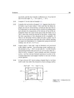
Figure 2.23 Configuration for
Problem 2.9.
90 Chapter 2: Heat conduction, thermal resistance, and the overall heat transfer coefficient
(U = 300 W/m
2
K) with steam condensing at 120
◦

C on its back.
Determine (a) q at the entrance; (b) the rate of increase of tem-
perature of the fluid with x at the entrance; (c) the temperature
and heat flux 2 m downstream. [(c): T
2m
= 89.7
◦
C.]
2.15 An isothermal sphere 3 cm in diameter is kept at 80
◦
Cina
large clay region. The temperature of the clay far from the
sphere is kept at 10
◦
C. How much heat must be supplied to
the sphere to maintain its temperature if k
clay
= 1.28 W/m·K?
(Hint: You must solve the boundary value problem not in the
sphere but in the clay surrounding it.) [Q = 16.9 W.]
2.16 Is it possible to increase the heat transfer from a convectively
cooled isothermal sphere by adding insulation? Explain fully.
2.17 A wall consists of layers of metals and plastic with heat trans-
fer coefficients on either side. U is 255 W/m
2
K and the overall
temperature difference is 200
◦
C. One layer in the wall is stain-
less steel (k = 18 W/m·K) 3 mm thick. What is ∆T across the

stainless steel?
2.18 A 1% carbon-steel sphere 20 cm in diameter is kept at 250
◦
Con
the outside. It has an 8 cm diameter cavity containing boiling
water (
h
inside
is very high) which is vented to the atmosphere.
What is Q through the shell?
2.19 A slab is insulated on one side and exposed to a surround-
ing temperature, T
∞
, through a heat transfer coefficient on the
other. There is nonuniform heat generation in the slab such
that
˙
q =[A (W/m
4
)][x (m)], where x = 0 at the insulated wall
and x = L at the cooled wall. Derive the temperature distribu-
tion in the slab.
2.20 800 W/m
3
of heat is generated within a 10 cm diameter nickel-
steel sphere for which k = 10 W/m·K. The environment is at
20
◦
C and there is a natural convection heat transfer coefficient
of 10 W/m

2
K around the outside of the sphere. What is its
center temperature at the steady state? [21.37
◦
C.]
2.21 An outside pipe is insulated and we measure its temperature
with a thermocouple. The pipe serves as an electrical resis-
tance heater, and
˙
q is known from resistance and current mea-
Problems 91
surements. The inside of the pipe is cooled by the flow of liq-
uid with a known bulk temperature. Evaluate the heat transfer
coefficient,
h, in terms of known information. The pipe dimen-
sions and properties are known. [Hint: Remember that
h is not
known and we cannot use a boundary condition of the third
kind at the inner wall to get T(r).]
2.22 Consider the hot water heater in Problem 1.11. Suppose that it
is insulated with 2 cm of a material for which k = 0.12 W/m·K,
and suppose that
h =16W/m
2
K. Find (a) the time constant
T for the tank, neglecting the casing and insulation; (b) the
initial rate of cooling in
◦
C/h; (c) the time required for the water
to cool from its initial temperature of 75

◦
Cto40
◦
C; (d) the
percentage of additional heat loss that would result if an outer
casing for the insulation were held on by eight steel rods, 1 cm
in diameter, between the inner and outer casings.
2.23 A slab of thickness L is subjected to a constant heat flux, q
1
,on
the left side. The right-hand side if cooled convectively by an
environment at T
∞
. (a) Develop a dimensionless equation for
the temperature of the slab. (b) Present dimensionless equa-
tion for the left- and right-hand wall temperatures as well. (c)
If the wall is firebrick, 10 cm thick, q
1
is 400 W/m
2
, h =20
W/m
2
K, and T
∞
=20
◦
C, compute the lefthand and righthand
temperatures.
2.24 Heat flows steadily through a stainless steel wall of thickness

L
ss
= 0.06 m, with a variable thermal conductivity of k
ss
= 1.67 +
0.0143 T(
◦
C). It is partially insulated on the right side with glass
wool of thickness L
gw
= 0.1 m, with a thermal conductivity
of k
gw
= 0.04. The temperature on the left-hand side of the
stainless stell is 400
◦
Cand on the right-hand side if the glass
wool is 100
◦
C. Evaluate q and T
i
.
2.25 Rework Problem 1.29 with a heat transfer coefficient,
h
o
=40
W/m
2
K on the outside (i.e., on the cold side).
2.26 A scientist proposes an experiment for the space shuttle in

which he provides underwater illumination in a large tank of
water at 20
◦
C, usinga3cmdiameter spherical light bulb. What
is the maximum wattage of the bulb in zero gravity that will
not boil the water?
92 Chapter 2: Heat conduction, thermal resistance, and the overall heat transfer coefficient
2.27 A cylindrical shell is made of two layers– an inner one with
inner radius = r
i
and outer radius = r
c
and an outer one with
inner radius = r
c
and outer radius = r
o
. There is a contact
resistance, h
c
, between the shells. The materials are different,
and T
1
(r = r
i
) = T
i
and T
2
(r = r

o
) = T
o
. Derive an expression
for the inner temperature of the outer shell (T
2
c
).
2.28 A 1 kW commercial electric heating rod, 8 mm in diameter and
0.3 m long, is to be used in a highly corrosive gaseous environ-
ment. Therefore, it has to be provided with a cylindrical sheath
of fireclay. The gas flows by at 120
◦
C, and h is 230 W/m
2
K out-
side the sheath. The surface of the heating rod cannot exceed
800
◦
C. Set the maximum sheath thickness and the outer tem-
perature of the fireclay. [Hint: use heat flux and temperature
boundary conditions to get the temperature distribution. Then
use the additional convective boundary condition to obtain the
sheath thickness.]
2.29 A very small diameter, electrically insulated heating wire runs
down the center of a 7.5 mm diameter rod of type 304 stain-
less steel. The outside is cooled by natural convection (
h = 6.7
W/m
2

K) in room air at 22
◦
C. If the wire releases 12 W/m, plot
T
rod
vs. radial position in the rod and give the outside temper-
ature of the rod. (Stop and consider carefully the boundary
conditions for this problem.)
2.30 A contact resistance experiment involves pressing two slabs of
different materials together, putting a known heat flux through
them, and measuring the outside temperatures of each slab.
Write the general expression for h
c
in terms of known quanti-
ties. Then calculate h
c
if the slabs are 2 cm thick copper and
1.5 cm thick aluminum, if q is 30,000 W/m
2
, and if the two
temperatures are 15
◦
C and 22.1
◦
C.
2.31 A student working heat transfer problems late at night needs
a cup of hot cocoa to stay awake. She puts milk in a pan on an
electric stove and seeks to heat it as rapidly as she can, without
burning the milk, by turning the stove on high and stirring the
milk continuously. Explain how this works using an analogous

electric circuit. Is it possible to bring the entire bulk of the milk
up to the burn temperature without burning part of it?
Problems 93
2.32 A small, spherical hot air balloon, 10 m in diameter, weighs
130 kg with a small gondola and one passenger. How much
fuel must be consumed (in kJ/h) if it is to hover at low altitude
in still 27
◦
C air? (h
outside
= 215 W/m
2
K, as the result of natural
convection.)
2.33 A slab of mild steel, 4 cm thick, is held at 1,000
◦
C on the back
side. The front side is approximately black and radiates to
black surroundings at 100
◦
C. What is the temperature of the
front side?
2.34 With reference to Fig. 2.3, develop an empirical equation for
k(T ) for ammonia vapor. Then imagine a hot surface at T
w
parallel with a cool horizontal surface at a distance H below it.
Develop equations for T(x)and q. Compute q if T
w
= 350
◦

C,
T
cool
= −5
◦
C, and H = 0.15 m.
2.35 A type 316 stainless steel pipe hasa6cminside diameter and
an 8 cm outside diameter witha2mmlayer of 85% magnesia
insulation around it. Liquid at 112
◦
C flows inside, so h
i
= 346
W/m
2
K. The air around the pipe is at 20
◦
C, and h
0
= 6 W/m
2
K.
Calculate U based on the inside area. Sketch the equivalent
electrical circuit, showing all known temperatures. Discuss
the results.
2.36 Two highly reflecting, horizontal plates are spaced 0.0005 m
apart. The upper one is kept at 1000
◦
C and the lower one at
200

◦
C. There is air in between. Neglect radiation and compute
the heat flux and the midpoint temperature in the air. Use a
power-law fit of the form k = a(T
◦
C)
b
to represent the air data
in Table A.6.
2.37 A 0.1 m thick slab with k = 3.4 W/m·K is held at 100
◦
Conthe
left side. The right side is cooled with air at 20
◦
C through a
heat transfer coefficient, and
h = (5.1 W/m
2
(K)
−5/4
)(T
wall
−
T
∞
)
1/4
. Find q and T
wall
on the right.

2.38 Heat is generated at 54,000 W/m
3
in a 0.16 m diameter sphere.
The sphere is cooled by natural convection with fluid at 0
◦
C,
and
h = [2 + 6(T
surface
− T
∞
)
1/4
] W/m
2
K, k
sphere
= 9 W/m·K.
Find the surface temperature and center temperature of the
sphere.
94 Chapter 2: Heat conduction, thermal resistance, and the overall heat transfer coefficient
2.39 Layers of equal thickness of spruce and pitch pine are lami-
nated to make an insulating material. How should the lamina-
tions be oriented in a temperature gradient to achieve the best
effect?
2.40 The resistances of a thick cylindrical layer of insulation must
be increased. Will Q be lowered more by a small increase of
the outside diameter or by the same decrease in the inside
diameter?
2.41 You are in charge of energy conservation at your plant. There

is a 300 m run of 6 in. O.D. pipe carrying steam at 250
◦
C. The
company requires that any insulation must pay for itself in
one year. The thermal resistances are such that the surface of
the pipe will stay close to 250
◦
C in air at 25
◦
C when h = 10
W/m
2
K. Calculate the annual energy savings in kW·h that will
result ifa1inlayer of 85% magnesia insulation is added. If
energy is worth 6 cents per kW·h and insulation costs $75 per
installed linear meter, will the insulation pay for itself in one
year?
2.42 An exterior wall of a wood-frame house is typically composed,
from outside to inside, of a layer of wooden siding, a layer
glass fiber insulation, and a layer of gypsum wall board. Stan-
dard glass fiber insulation has a thickness of 3.5 inch and a
conductivity of 0.038 W/m·K. Gypsum wall board is normally
0.50 inch thick with a conductivity of 0.17 W/m·K, and the sid-
ing can be assumed to be 1.0 inch thick with a conductivity of
0.10 W/m·K.
a. Find the overall thermal resistance of such a wall (in K/W)
if it has an area of 400 ft
2
.
b. Convection and radiation processes on the inside and out-

side of the wall introduce more thermal resistance. As-
suming that the effective outside heat transfer coefficient
(accounting for both convection and radiation) is
h
o
=20
W/m
2
K and that for the inside is h
i
=10W/m
2
K, deter-
mine the total thermal resistance for heat loss from the
indoors to the outdoors. Also obtain an overall heat trans-
fer coefficient, U,inW/m
2
K.
Problems 95
c. If the interior temperature is 20
◦
C and the outdoor tem-
perature is −5
◦
C, find the heat loss through the wall in
watts and the heat flux in W/m
2
.
d. Which of the five thermal resistances is dominant?
2.43 We found that the thermal resistance of a cylinder was R

t
cyl
=
(1/2πkl)ln(r
o
/r
i
).Ifr
o
= r
i
+δ, show that the thermal resis-
tance of a thin-walled cylinder (δ  r
i
) can be approximated
by that for a slab of thickness δ. Thus, R
t
thin
= δ/(kA
i
), where
A
i
= 2πr
i
l is the inside surface area of the cylinder. How
much error is introduced by this approximation if δ/r
i
= 0.2?
[Hint: Use a Taylor series.]

2.44 A Gardon gage measures a radiation heat flux by detecting a
temperature difference [2.10]. The gage consists of a circular
constantan membrane of radius R, thickness t, and thermal
conductivity k
ct
which is joined to a heavy copper heat sink
at its edges. When a radiant heat flux q
rad
is absorbed by the
membrane, heat flows from the interior of the membrane to
the copper heat sink at the edge, creating a radial tempera-
ture gradient. Copper leads are welded to the center of the
membrane and to the copper heat sink, making two copper-
constantan thermocouple junctions. These junctions measure
the temperature difference ∆T between the center of the mem-
brane, T(r = 0), and the edge of the membrane, T(r = R).
The following approximations can be made:
• The membrane surface has been blackened so that it ab-
sorbs all radiation that falls on it
• The radiant heat flux is much larger than the heat lost
from the membrane by convection or re-radiation. Thus,
all absorbed radiant heat is removed from the membrane
by conduction to the copper heat sink, and other loses
can be ignored
• The gage operates in steady state
• The membrane is thin enough (t  R) that the tempera-
ture in it varies only with r , i.e., T = T(r) only.
Answer the following questions.
96 Chapter 2: Heat conduction, thermal resistance, and the overall heat transfer coefficient
a. For a fixed copper heat sink temperature, T(r = R), sketch

the shape of the temperature distribution in the mem-
brane, T(r), for two arbitrary heat radiant fluxes q
rad
1
and q
rad
2
, where q
rad
1
>q
rad
2
.
b. Find the relationship between the radiant heat flux, q
rad
,
and the temperature difference obtained from the ther-
mocouples, ∆T . Hint: Treat the absorbed radiant heat
flux as if it were a volumetric heat source of magnitude
q
rad
/t (W/m
3
).
2.45 You have a 12 oz. (375 mL) can of soda at room temperature
(70
◦
F) that you would like to cool to 45
◦

F before drinking. You
rest the can on its side on the plastic rods of the refrigerator
shelf. The can is 2.5 inches in diameter and 5 inches long.
The can’s emissivity is ε = 0.4 and the natural convection heat
transfer coefficient around it is a function of the temperature
difference between the can and the air:
h = 2 ∆T
1/4
for ∆T in
kelvin.
Assume that thermal interactions with the refrigerator shelf
are negligible and that buoyancy currents inside the can will
keep the soda well mixed.
a. Estimate how long it will take to cool the can in the refrig-
erator compartment, which is at 40
◦
F.
b. Estimate how long it will take to cool the can in the freezer
compartment, which is at 5
◦
F.
c. Are your answers for parts 1 and 2 the same? If not, what
is the main reason that they are different?
References
[2.1] W. M. Rohsenow and J. P. Hartnett, editors. Handbook of Heat
Transfer. McGraw-Hill Book Company, New York, 1973.
[2.2] R. F. Wheeler. Thermal conductance of fuel element materials.
USAEC Rep. HW-60343, April 1959.
[2.3] M. M. Yovanovich. Recent developments in thermal contact, gap
and joint conductance theories and experiment. In Proc. Eight Intl.

Heat Transfer Conf., volume 1, pages 35–45. San Francisco, 1986.
References 97
[2.4] C. V. Madhusudana. Thermal Contact Conductance. Springer-
Verlag, New York, 1996.
[2.5] R. A. Parsons, editor. 1993 ASHRAE Handbook—Fundamentals.
American Society of Heating, Refrigerating, and Air-Conditioning
Engineers, Inc., Altanta, 1993.
[2.6] R.K. Shah and D.P. Sekulic. Heat exchangers. In W. M. Rohsenow,
J. P. Hartnett, and Y. I. Cho, editors, Handbook of Heat Transfer,
chapter 17. McGraw-Hill, New York, 3rd edition, 1998.
[2.7] Tubular Exchanger Manufacturer’s Association. Standards of
Tubular Exchanger Manufacturer’s Association. New York, 4th and
6th edition, 1959 and 1978.
[2.8] H. Müller-Steinhagen. Cooling-water fouling in heat exchangers.
In T.F. Irvine, Jr., J. P. Hartnett, Y. I. Cho, and G. A. Greene, editors,
Advances in Heat Transfer, volume 33, pages 415–496. Academic
Press, Inc., San Diego, 1999.
[2.9] W. J. Marner and J.W. Suitor. Fouling with convective heat transfer.
In S. Kakaç, R. K. Shah, and W. Aung, editors, Handbook of Single-
Phase Convective Heat Transfer, chapter 21. Wiley-Interscience,
New York, 1987.
[2.10] R. Gardon. An instrument for the direct measurement of intense
thermal radiation. Rev. Sci. Instr., 24(5):366–371, 1953.
Most of the ideas in Chapter 2 are also dealt with at various levels in
the general references following Chapter 1.

3. Heat exchanger design
The great object to be effected in the boilers of these engines is, to keep
a small quantity of water at an excessive temperature, by means of a
small amount of fuel kept in the most active state of combustion No

contrivance can be less adapted for the attainment of this end than one or
two large tubes traversing the boiler, as in the earliest locomotive engines.
The Steam Engine Familiarly Explained and Illustrated,
Dionysus Lardner, 1836
3.1 Function and configuration of heat exchangers
The archetypical problem that any heat exchanger solves is that of get-
ting energy from one fluid mass to another, as we see in Fig. 3.1. A simple
or composite wall of some kind divides the two flows and provides an
element of thermal resistance between them. There is an exception to
this configuration in the direct-contact form of heat exchanger. Figure
3.2 shows one such arrangement in which steam is bubbled into water.
The steam condenses and the water is heated at the same time. In other
arrangements, immiscible fluids might contact each other or nonconden-
sible gases might be bubbled through liquids.
This discussion will be restricted to heat exchangers with a dividing
wall between the two fluids. There is an enormous variety of such config-
urations, but most commercial exchangers reduce to one of three basic
types. Figure 3.3 shows these types in schematic form. They are:
• The simple parallel or counterflow configuration. These arrange-
ments are versatile. Figure 3.4 shows how the counterflow arrange-
ment is bent around in a so-called Heliflow compact heat exchanger
configuration.
• The shell-and-tube configuration. Figure 3.5 shows the U-tubes of
a two-tube-pass, one-shell-pass exchanger being installed in the
99
100 Heat exchanger design §3.1
Figure 3.1 Heat exchange.
supporting baffles. The shell is yet to be added. Most of the re-
ally large heat exchangers are of the shell-and-tube form.
• The cross-flow configuration. Figure 3.6 shows typical cross-flow

units. In Fig. 3.6a and c, both flows are unmixed. Each flow must
stay in a prescribed path through the exchanger and is not allowed
to “mix” to the right or left. Figure 3.6b shows a typical plate-fin
cross-flow element. Here the flows are also unmixed.
Figure 3.7, taken from the standards of the Tubular Exchanger Manu-
facturer’s Association (TEMA) [3.1], shows four typical single-shell-pass
heat exchangers and establishes nomenclature for such units.
These pictures also show some of the complications that arise in
translating simple concepts into hardware. Figure 3.7 shows an exchan-
ger with a single tube pass. Although the shell flow is baffled so that it
crisscrosses the tubes, it still proceeds from the hot to cold (or cold to
hot) end of the shell. Therefore, it is like a simple parallel (or counter-
flow) unit. The kettle reboiler in Fig. 3.7d involves a divided shell-pass
flow configuration over two tube passes (from left to right and back to the
“channel header”). In this case, the isothermal shell flow could be flowing
in any direction—it makes no difference to the tube flow. Therefore, this
exchanger is also equivalent to either the simple parallel or counterflow
configuration.
§3.1 Function and configuration of heat exchangers 101
Figure 3.2 A direct-contact heat exchanger.
Notice that a salient feature of shell-and-tube exchangers is the pres-
ence of baffles. Baffles serve to direct the flow normal to the tubes. We
find in Part III that heat transfer from a tube to a flowing fluid is usually
better when the flow moves across the tube than when the flow moves
along the tube. This augmentation of heat transfer gives the complicated
shell-and-tube exchanger an advantage over the simpler single-pass par-
allel and counterflow exchangers.
However, baffles bring with them a variety of problems. The flow pat-
terns are very complicated and almost defy analysis. A good deal of the
shell-side fluid might unpredictably leak through the baffle holes in the

axial direction, or it might bypass the baffles near the wall. In certain
shell-flow configurations, unanticipated vibrational modes of the tubes
might be excited. Many of the cross-flow configurations also baffle the
fluid so as to move it across a tube bundle. The plate-and-fin configura-
tion (Fig. 3.6b) is such a cross-flow heat exchanger.
In all of these heat exchanger arrangements, it becomes clear that a
dramatic investment of human ingenuity is directed towards the task of
augmenting the heat transfer from one flow to another. The variations
are endless, as you will quickly see if you try Experiment 3.1.
Experiment 3.1
Carry a notebook with you for a day and mark down every heat ex-
changer you encounter in home, university, or automobile. Classify each
according to type and note any special augmentation features.
The analysis of heat exchangers first becomes complicated when we
account for the fact that two flow streams change one another’s temper-
Figure 3.3 The three basic types of heat exchangers.
102
§3.2 Evaluation of the mean temperature difference in a heat exchanger 103
Figure 3.4 Heliflow compact counterflow heat exchanger.
(Photograph coutesy of Graham Manufacturing Co., Inc.,
Batavia, New York.)
ature. It is to the problem of predicting an appropriate mean tempera-
ture difference that we address ourselves in Section 3.2. Section 3.3 then
presents a strategy to use when this mean cannot be determined initially.
3.2 Evaluation of the mean temperature difference
in a heat exchanger
Logarithmic mean temperature difference (LMTD)
To begin with, we take U to be a constant value. This is fairly reasonable
in compact single-phase heat exchangers. In larger exchangers, particu-
larly in shell-and-tube configurations and large condensers, U is apt to

vary with position in the exchanger and/or with local temperature. But
in situations in which U is fairly constant, we can deal with the varying
temperatures of the fluid streams by writing the overall heat transfer in
terms of a mean temperature difference between the two fluid streams:
Q = UA∆T
mean
(3.1)
Figure 3.5 Typical commercial one-shell-pass, two-tube-pass
heat exchangers.
104
Figure 3.6 Several commercial cross-flow heat exchangers.
(Photographs courtesy of Harrison Radiator Division, General
Motors Corporation.)
105
Figure 3.7 Four typical heat exchanger configurations (contin-
ued on next page). (Drawings courtesy of the Tubular Exchan-
ger Manufacturers’ Association.)
106
§3.2 Evaluation of the mean temperature difference in a heat exchanger 107
Figure 3.7 Continued
Our problem then reduces to finding the appropriate mean temperature
difference that will make this equation true. Let us do this for the simple
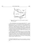
parallel and counterflow configurations, as sketched in Fig. 3.8.
The temperature of both streams is plotted in Fig. 3.8 for both single-
pass arrangements—the parallel and counterflow configurations—as a
function of the length of travel (or area passed over). Notice that, in the
parallel-flow configuration, temperatures tend to change more rapidly
with position and less length is required. But the counterflow arrange-
ment achieves generally more complete heat exchange from one flow to
the other.

Figure 3.9 shows another variation on the single-pass configuration.
This is a condenser in which one stream flows through with its tempera-
108 Heat exchanger design §3.2
Figure 3.8 The temperature variation through single-pass
heat exchangers.
ture changing, but the other simply condenses at uniform temperature.
This arrangement has some special characteristics, which we point out
shortly.
The determination of ∆T
mean
for such arrangements proceeds as fol-
lows: the differential heat transfer within either arrangement (see Fig. 3.8)
is
dQ = U∆TdA=−(
˙
mc
p
)
h
dT
h
=±(
˙
mc
p
)
c
dT
c
(3.2)

where the subscripts h and c denote the hot and cold streams, respec-
tively; the upper and lower signs are for the parallel and counterflow
cases, respectively; and dT denotes a change from left to right in the
exchanger. We give symbols to the total heat capacities of the hot and
cold streams:
C
h
≡ (
˙
mc
p
)
h
W/K and C
c
≡ (
˙
mc
p
)
c
W/K (3.3)
Thus, for either heat exchanger, ∓C
h
dT
h
= C
c
dT
c

. This equation can
be integrated from the lefthand side, where T
h
= T
h
in
and T
c
= T
c
in
for
§3.2 Evaluation of the mean temperature difference in a heat exchanger 109
Figure 3.9 The temperature distribution through a condenser.
parallel flow or T
h
= T
h
in
and T
c
= T
c
out
for counterflow, to some arbitrary
point inside the exchanger. The temperatures inside are thus:
parallel flow: T
h
= T
h

in
−
C
c
C
h
(T
c
−T
c
in
) = T
h
in
−
Q
C
h
counterflow: T
h
= T
h
in
−
C
c
C
h
(T
c

out
−T
c
) = T
h
in
−
Q
C
h
(3.4)
where Q is the total heat transfer from the entrance to the point of inter-
est. Equations (3.4) can be solved for the local temperature differences:
∆T
parallel
= T
h
−T
c
= T
h
in
−

1 +
C
c
C
h


T
c
+
C
c
C
h
T
c
in
∆T
counter
= T
h
−T
c
= T
h
in
−

1 −
C
c
C
h

T
c
−

C
c
C
h
T
c
out
(3.5)
110 Heat exchanger design §3.2
Substitution of these in dQ = C
c
dT
c
= U∆TdAyields
UdA
C
c




parallel
=
dT
c

−

1 +
C

c
C
h

T
c
+
C
c
C
h
T
c
in
+T
h
in

UdA
C
c




counter
=
dT
c


−

1 −
C
c
C
h

T
c
−
C
c
C
h
T
c
out
+T
h
in

(3.6)
Equations (3.6) can be integrated across the exchanger:

A
0
U
C
c

dA =

T
c
out
T
c
in
dT
c
[−−−]
(3.7)
If U and C
c
can be treated as constant, this integration gives
parallel: ln





−

1 +
C
c
C
h

T

c
out
+
C
c
C
h
T
c
in
+T
h
in
−

1 +
C
c
C
h

T
c
in
+
C
c
C
h
T

c
in
+T
h
in





=−
UA
C
c

1 +
C
c
C
h

counter: ln





−

1 −

C
c
C
h

T
c
out
−
C
c
C
h
T
c
out
+T
h
in
−

1 −
C
c
C
h

T
c
in

−
C
c
C
h
T
c
out
+T
h
in





=−
UA
C
c

1 −
C
c
C
h

(3.8)
If U were variable, the integration leading from eqn. (3.7) to eqns. (3.8)
is where its variability would have to be considered. Any such variability

of U can complicate eqns. (3.8) terribly. Presuming that eqns. (3.8) are
valid, we can simplify them with the help of the definitions of ∆T
a
and
∆T
b
, given in Fig. 3.8:
parallel: ln

(1 +C
c
/C
h
)(T
c
in
−T
c
out
) +∆T
b
∆T
b

=−UA

1
C
c
+

1
C
h

counter: ln
∆T
a
(−1 +C
c
/C
h
)(T
c
in
−T
c
out
) +∆T
a
=−UA

1
C
c
−
1
C
h

(3.9)

Conservation of energy (Q
c
= Q
h
) requires that
C
c
C
h
=−
T
h
out
−T
h
in
T
c
out
−T
c
in
(3.10)
§3.2 Evaluation of the mean temperature difference in a heat exchanger 111
Then eqn. (3.9) and eqn. (3.10) give
parallel: ln







∆T
a
−∆T
b
  
(T
c
in
−T
c
out
) +(T
h
out
−T
h
in
) +∆T
b
∆T
b






= ln


∆T
a
∆T
b

=−UA

1
C
c
+
1
C
h

counter: ln

∆T
a
∆T
b
−∆T
a
+∆T
a

= ln

∆T

a
∆T
b

=−UA

1
C
c
−
1
C
h

(3.11)
Finally, we write 1/C
c
= (T
c
out
− T
c
in
)/Q and 1/C
h
= (T
h
in
− T
h

out
)/Q on
the right-hand side of either of eqns. (3.11) and get for either parallel or
counterflow,
Q = UA

∆T
a
−∆T
b
ln(∆T
a
/∆T
b
)

(3.12)
The appropriate ∆T
mean
for use in eqn. (3.11) is thus the logarithmic mean
temperature difference (LMTD):
∆T
mean
= LMTD ≡
∆T
a
−∆T
b
ln


∆T
a
∆T
b

(3.13)
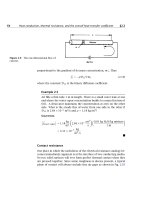
Example 3.1
The idea of a logarithmic mean difference is not new to us. We have
already encountered it in Chapter 2. Suppose that we had asked,
“What mean radius of pipe would have allowed us to compute the
conduction through the wall of a pipe as though it were a slab of
thickness L = r
o
−r
i
?” (see Fig. 3.10). To answer this, we compare
Q = kA
∆T
L
= 2πkl∆T

r
mean
r
o
−r
i

with eqn. (2.21):
Q = 2πkl∆T

1
ln(r
o
/r
i
)
112 Heat exchanger design §3.2
Figure 3.10 Calculation of the mean radius for heat conduc-
tion through a pipe.
It follows that
r
mean
=
r
o
−r
i
ln(r
o
/r
i
)
= logarithmic mean radius
Example 3.2
Suppose that the temperature difference on either end of a heat ex-
changer, ∆T
a
, and ∆T
b
, are equal. Clearly, the effective ∆T must equal

∆T
a
and ∆T
b
in this case. Does the LMTD reduce to this value?
Solution. If we substitute ∆T
a
= ∆T
b
in eqn. (3.13), we get
LMTD =
∆T
b
−∆T
b
ln(∆T
b
/∆T
b
)
=
0
0
= indeterminate
Therefore it is necessary to use L’Hospital’s rule:
limit
∆T
a
→∆T
b

∆T
a
−∆T
b
ln(∆T
a
/∆T
b
)
=
∂
∂∆T
a
(∆T
a
−∆T
b
)




∆T
a
=∆T
b
∂
∂∆T
a
ln


∆T
a
∆T
b






∆T
a
=∆T
b
=

1
1/∆T
a






∆T
a
=∆T
b

= ∆T
a
= ∆T
b
§3.2 Evaluation of the mean temperature difference in a heat exchanger 113
It follows that the LMTD reduces to the intuitively obvious result in
the limit.
Example 3.3
Water enters the tubes of a small single-pass heat exchanger at 20
◦
C
and leaves at 40
◦
C. On the shell side, 25 kg/min of steam condenses at
60
◦
C. Calculate the overall heat transfer coefficient and the required
flow rate of water if the area of the exchanger is 12 m
2
. (The latent
heat, h
fg
, is 2358.7 kJ/kg at 60
◦
C.)
Solution.
Q =
˙
m
condensate

·h
fg



60
◦
C
=
25(2358.7)
60
= 983 kJ/s
and with reference to Fig. 3.9, we can calculate the LMTD without
naming the exchanger “parallel” or “counterflow”, since the conden-
sate temperature is constant.
LMTD =
(60 −20) −(60 −40)
ln

60 −20
60 −40

= 28.85 K
Then
U =
Q
A(LMTD)
=
983(1000)
12(28.85)

= 2839 W/m
2
K
and
˙
m
H
2
O
=
Q
c
p
∆T
=
983, 000
4174(20)
= 11.78 kg/s
Extended use of the LMTD
Limitations. There are two basic limitations on the use of an LMTD.
The first is that it is restricted to the single-pass parallel and counter-
flow configurations. This restriction can be overcome by adjusting the
LMTD for other configurations—a matter that we take up in the following
subsection.