Atomic Force Microscopy in Cell Biology Episode 1 Part 5 doc

84 Lydataki et al.
Changes in the Sperm Surface Structure 85
85
7
AFM Study of Surface Structure Changes
in Mouse Spermatozoa Associated With Maturation
Hiroko Takano and Kazuhiro Abe
1. Introduction
If a sample has a comparatively even surface and is fixed on a sample stage,
atomic force microscopy (AFM) will give a clear image of the surface struc-
ture at subnanometer level (1,2). Because a sperm head is flat and can be
attached on the slide glass firmly after it is fixed, we consider that AFM is the
competent tool for the study of the sperm surface structure.
Spermatozoa are produced in the testis and transferred into the epididymis.
In the epididymis, they acquire a fertilization ability and mobility, which is
called sperm maturation (3). It has been proved biochemically and immunocy-
tochemically that glycoproteins on or in the sperm plasma membrane are
altered, masked, or replaced by new glycoproteins of epididymal origin in the
epididymal duct (4–6). These changes are considered to be necessary for fer-
tilization (3,7). Thus, it is probable that the sperm surface structure changes
progressively in the epididymal duct (8). We reported the changes in the sur-
face structure of the spermatozoa in the hamster epididymis by AFM (9). Sub-
sequently, we have studied the surface structure of the spermatozoa from mouse
epididymis by AFM. In these studies we developed several tricks for improv-
ing AFM images. In this chapter, we will show our recent results and the mate-
rials and methods used , including the tricks we learned in these studies.
Histologically, the mouse epididymis is divided into five regions (segments
I–V) in adult male mice (Fig. 1; refs. 10,11). These segments perform different
roles in the process of sperm maturation (12). Spermatozoa are immature in
segment I but mature in segment V (13). The epithelial cells in segment II
appear to secrete glycoproteins for sperm maturation (10,14,15), so we exam-

ined the segments I, II, and V of the mouse spermatozoa by AFM.
From:
Methods in Molecular Biology, vol. 242: Atomic Force Microscopy: Biomedical Methods and Applications
Edited by: P. C. Braga and D. Ricci © Humana Press Inc., Totowa, NJ
86 Takano and Abe
The surface of the sperm head is classically divided into two domains, the
acrosomal region and postacrosomal region (Fig. 2). The acrosomal region is
subdivided into the acrosomal cap and equatorial segment (Fig. 2). These
domains play the different roles at fertilization (16,17). The plasma membrane
of the equatorial segment is maintained after acrosome reaction and fuses with
Fig. 1. Schematic diagram of the histological segmentation of the mouse epididy-
mis. ED, efferent duct; I–V, epididymal segments; DD, deferent duct.
Fig. 2. Diagrams traced from the AFM images of the mouse spermatozoa from
segments I (left), II (middle), and V (right). AC, acrosomal cap; ES, equatorial seg-
ment; PAR, post-acrosomal region.
Changes in the Sperm Surface Structure 87
the plasma membrane of an oocyte at fertilization (3). Because of this, our
study focused on the changes in the surface structure of the equatorial segment.
Dynamic force mode AFM, as used in our laboratory, provides images in
constant height mode, amplitude mode, and phase mode. Images in constant
height mode offer the topographical information of the sample height (Fig. 3).
Those in amplitude mode and phase mode offer well-defined contours of the
projections and hollows based on the changes in oscillation amplitude and
phase, respectively (Figs. 4–6). Using a combination of these modes, the sperm
head was shown to be covered with particles whose diameter was < 100 nm.
The size of the surface particles differed between the acrosomal region and
postacrosomal region in the same spermatozoon. Particularly, the particles cov-
ering the equatorial segment changed in size dramatically during the passage
through the epididymal duct (Figs. 4–6). The surface of the equatorial segment
was covered with the particles of 20–50 nm in diameter in segment I, 50–80 nm

in segment II, and 20 nm in segment V. These size differences generated the
different morphological surface features among the spermatozoa from seg-
ments I, II, and V (Figs. 4–6). Because the epithelial cells in segment II appear
to secrete acid glycoproteins, which play a role as a sperm maturing factor
(10,14,15), large particles covering the segment II sperm surface may be gly-
coproteins secreted from the epithelial cells in segment II.
AFM images also demonstrated the changes in shape of the acrosomal cap.
The acrosome cap is flat and wider in the immature spermatozoa from seg-
ments I and II than in mature spermatozoa from segment V (Figs. 2 and 3A
through 6A). Thus, an application of AFM for the study of the surface structure
of the mouse spermatozoa brought us noteworthy new findings.
2. Materials
1. A mature male dd-mouse at 90 days of age.
2. Modified tyrode solution (this medium is used for making sperm suspension and
for washing spermatozoa by centrifugation): 500 mL distilled water, 2.05 g NaCl,
0.1 g KCl, 0.1 g CaCl
2
(anhyd.), 0.05 g MgCl
2
/H
2
O, 0.025 g NaH
2
PO
4
/H
2
O, 1.5 g
NaHCO
3

, approx pH 8.0. This stock solution can be used for one month if stored
at 4°C.
3. Fixative: 2% glutaraldehyde in 0.1 M cacodylate buffer.
4. Ethyl alcohol (anhyd.).
5. 3-methylbutyl acetate.
6. Nitrogen gas.
7. A double-edged razor.
8. Small vials.
9. Test tubes.
10. Test-tube stand.
11. Disposable pipets.
12. Plastic dishes for ethyl alcohol.
88 Takano and Abe
Fig. 3. AFM image in constant force mode of epididymal segment I.
Fig. 4. AFM image in amplitude mode of the same spermatozoon as in Fig. 3.
Fig. 5. AFM image in amplitude mode of the spermatozoon from segment II.
Fig. 6. AFM image in amplitude mode of the spermatozoon from segment V.
Changes in the Sperm Surface Structure 89
13 A glass dish for 3-butyl-ethyl acetate.
14. Micro slide glass coated with adhesive material (Superfrost, Matunami Glass
IND., LTD, Japan).
a. Cut the micro slide glass into 7-mm squares.
b. Mark the surface of one side of of the slide glass squares with the glass cutter
to distinguish the side of the sperm attachment.
15. Centrifugal separator.
16. Critical point drier.
17. AFM.
a. Probe station/Unit SPI3800 /SPA300 (Seiko Instruments, Japan).
b. Scanner table (a maximum scan range is 20 µm × 20 µm × 3 µm, (x, y, z
direction).

c. Lever table (20 N/m).
d. Cantilever tips SI-DF20 (Seiko Instruments, Japan).
e. Optical microscope.
f. Antivibration platform and nitrogen gas bomb.
3. Methods
3.1. Preparation of Samples
1. Remove both sides of the epididymis from a mature dd-mouse. Separate the tis-
sue of segments I–V of the epididymis (Fig. 1; ref. 10).Cut tissue blocks of seg-
ments I, II, and V into small pieces with razors and place in the bottom of small
vials separately.
2. Pour 3 mL of medium into each small vial and make the small pieces of tissue
separate in the medium with tweezers. Wait a few minutes for spermatozoa to
submerge from the stumps of the epididymal duct.
3. Transfer 2 mL of sperm suspension to a centrifugal tube and centrifuge at 240g
for 8 min.
4. Pour 3 mL of medium into each centrifugal tube to wash the spermatozoa, and
centrifuge at 240g for 8 min twice more.
5. Fix the spermatozoa in 2% glutaraldehyde in 0.1 M cacodylate buffer solution for 1 h.
6. Adjust the total amount of the sperm suspension to be 0.3 mL with distilled water
after centrifugation.
7. Place one drop of sperm suspension on the slide glass square. As the glass is
coated with adhesive material, spermatozoa adhere to the surface of the glass in
5–10 min. Make 3 or 4 samples.
8. Move the slide glass in distilled water to allow the release of loosely-attached
spermatozoa from the slide glass.
9. Check the density of the spermatozoa on the slide glass under a light microscope.
10. Transfer the slide glass with spermatozoa in turn to 80 (5 min), 90 (5 min), 95
(5 min), and 100% (10 min, twice) ethyl alcohol solutions for dehydration.
Figs. 3–6. (facing page) AFM images of mouse epididymal spermatozoa. (B) and
(C) are enlarged images of (A). Bar is 2 µm in (A), 1 µm in (B), and 0.5 µm in (C).

90 Takano and Abe
11. Immerse the samples in 3-butyl-ethyl acetate solution for 15 min.
12. Put a sample in a cage and perform critical point drying.
3.2. Scanning Operation Method of Dynamic Force Mode (DFM)
1. Allow the nitrogen gas to flow into the antivibration platform.
2. Turn on the antivibration platform and CCD camera controller.
3. Turn on the light of the optical microscope.
4. Set the scanner table.
5. Turn on the power at the center of the front panel of SPI3800N probe station
controller.
6. Turn on the computer and the display. Microsoft Windows startup menu will
appear.
7. Double click the icon of Spise132 on the desktop to open the application for AFM.
8. Select “DFM” in “SPA300/400” frame and click “OK”; the main program,
SPIWin, will start.
9. Set the sample stage on the mount on top of the scanner.
10. Set the sample on the sample stage.
11. Select a spermatozoon and move it to the center of the eye field of the optical
microscope by hand.
12. Install the DFM cantilever holder with a DFM cantilever into the unit.
13. Select “CCD Monitor” in the setup menu to display “CCD”. Check the position
of the cantilever and the specimen by CCD image. Use the Move-in command
(Low or High) and set the distance between the sample and the cantilever at approx
0.1 mm (which corresponds to a 180°- rotation of the fine-focus dial of the optical
microscope).
14. Set the laser unit on SPA 300.
15. Adjust the laser light spot to be in right position.
a. Rotate adjustment knobs “Laser X” and “Laser Y” to put the laser light spot
on the top of the cantilever under the optical microscope.
b. Rotate adjustment knobs “Laser X” and “Laser Y” to maximize ADD output.

The maximum value of ADD output is around 5 or 13 depending on the can-
tilever.
c. Rotate adjustment knob “DIF” so that the output may be in the range from –1
to 1 V
d. Rotate adjustment knobs “DIF” and “FFM” so that the output may be in the
range from 0 to 1 V.
16. Measure the Q-curve.
a. Select “Q-curve” in the Scan menu to display “Q-curve Console.”
b. Put the initial value of the parameter of the Q-curve Console. One example
follows:
Freq. High 400 kHz
Low 1 kHz
Gain 1
Vib. Voltage 1 V
LPF 1 kHz
Changes in the Sperm Surface Structure 91
HPF 1 kHz
Time 5 s
c. Select “Left” in the Vib. Freq. frame.
d. Check “Phase,” “Calibration,” and “Auto Set.”
e. Click “Configuration” button to display configuration dialog.
f. Set the value of the auto set. “Amplitude” is 1.000 V and “Frequency” is
3.000 kHz.
g. Click “Start” to measure the Q-curve and the phase curve. Computer calcu-
lates the optimal value for the vibration frequency (operation point) immedi-
ately and displays the values with the Q-curve. An example follows:
Freq. High 128.410 kHz
Low 125.410 kHz
Gain 1.000
Vib. Voltage 1.511 V

LPF 1.0 kHz
HPF 1.0 kHz
Time 5 s
Vib. Freq. 126.800
Amplitude 1.068 V
Peak Freq. 126.918 kHz
∆F 0.335
Q 379.273
Phase –56.520°
h. Click “Close” to close, on the Q-curve Console
18. Approach the force area.
a. Select “Image” in the Scan menu to display “Approach” and “Scan Console.”
b. Preset the parameters in the Scan Console follows:
Amplitude Reference -0.101
I-gain 0.177, P-gain 0.0488, A-gain 0, S-gain 0
when the maximum ADD value is around 5.
I-gain 0.0592, P-gain 0.0122, A-gain 0, S-gain 0
when the maximum ADD value is around 13.
c. Open “Sub Console” to confirm the filter values for topography.
Data Type Topo (servo)
LPF 1.000 kHz, HPF 0.000 Hz, Range 1583.20 nm, Offset 0.715V
d. Approach the sample to the cantilever by using the Approach button.
e. Lower the value of the Amplitude Reference until the scanning voltage
becomes stable.
f. Make the Amplitude Reference 0.3–0.5 down from the value of getting stabil-
ity of the scanning voltage.
19. Separate the sample from the cantilever until the scanning voltage displays –20.
20. Turn off the laser light.
21. Insert the head of the spermatozoa under the tip of the cantilever under the optic
microscope.

22. Perform the test scan at 512 × 128 points in the area of 15,000 nm
2
at the scan
speed of 1 Hz.
92 Takano and Abe
23. Approach the force area by using the “Approach” button and click “Start.”
24. Execute steps 21–23 again when the object is not displayed in the canvas.
25. Change the rotation angle, center of the image, and scan area to get the proper
compositon. Use “Zoom” to change the center of the image.
26. Check the composition of the image by test scan.
27. Write the sample information in the column for comments.
28. Change the number of the scan points to 512 × 512.
29. The relation between “Scan Area” and “Scan Speed follows.”
Scan area (nm) Scan speed (Hz )
9,000 0.28
8,000 0.28
6,000 0.37
4,000 0.41
3,000 0.56
2,000 0.85
1,000 1.23
It takes 40 min to get an image of 9,000 nm square.
30. Start to scan.
31. Set the S-gain value between 3 and 8 if the image is improved by this.
32. Separate the sample from the cantilever after completing the scan.
33. Save the measured data into HDD or MO as soon as possible.
34. When all measurements are finished, close the SPIWin software and CCD monitor.
35. Shut down the system.
36. Turn off the light of the optical microscope.
37. Turn off the power of CCD camera controller and antivibration platform.

38. Stop nitrogen gas to flow to the antivibration platform.
39. Turn off the power at the center of the front panel of SPI3800N Probe station
controller.
4. Notes
1. When the ADD output does not move freely, readjust the position of the laser light on
the cantilever or the distance between the specimen and the cantilever to be adequate
(approx 0/1 mm).
2. The adequate value of the Amplitude Reference often moves in the minus direc-
tion during scanning. In this case the scanned image will become blurred and
disappear at last. To avoid this, the value of the Amplitude Reference is better set
0.3–0.5 lower than the value necessary to stabilize the scanning voltage.
3. Caution the following items to prevent the cantilever tip from damages.
a. Scanning should not be stopped on the way of image delineation, even if the
image is not good.
b. The rotation angle and the scan area of the image should not be changed when
the sample is in the force area.
c. When the computer freezes, the sample should be separated from the cantile-
ver by using up-down lever equipped in SPA300 before application is stopped.
d. FFM knob should not be rotated during scanning.
Changes in the Sperm Surface Structure 93
4. Pay attention to the appearance of double images or two or more triangle-shaped
particles arranged in the same direction, which reflect damage to the cantilever
tip. If these signs appear, replace the cantilever immediately.
5. When an image does not appear in the NC-force canvas, try again and you will
get the image.
6. A test scan is recommended after the scan area is changed because the scan posi-
tion often shifts after that.
7. When the scanning voltage shows 200, the following three reasons should be
taken into consideration.
a. The laser beam is now off.

b. The proper value of the amplitude reference is changed spontaneously to
minus direction. In this case remeasurement of Q-curve is effective.
c. FFM value is out of ±1.0 V.
8. Check the FFM value just before scanning, because FFM value is easy to change.
References
1. Ushiki, T., Hitomi, J., Ogura S., Umemoto, T., and Shigeno M. (1996) Atomic
force microscopy in histology and cytology. Arch. Histol. Cytol. 59, 421–431.
2. Tojima, T., Hatakeyama, D., Kawabata, K., Abe, K., and Ito, E. (1999) Reexami-
nation of fine surface topography of nerve cells revealed by atomic force micros-
copy. Bioimages 7, 89–94.
3. Yanagimachi, R. (1994) Mammalian fertilization, in The Physiology of Repro-
duction, Vol. 1, 2nd ed . (Knobil, E. and Neill, J. D., eds.), Raven Press, New
York, pp. 189–317.
4. Brooks, D. E. and Higgins, S. J. (1980) Characterization and androgen-depen-
dence of proteins associated with luminal fluid and spermatozoa in the rat epid-
idymis. J. Reprod. Fertil. 59, 363–375.
5. Jones, R., Pholpramool, C., Setchell, B. P., and Brown, C. R. (1981) Labelling of
membrane glycoproteins on rat spermatozoa collected from different regions of
the epididymis. Biochem J. 200, 457–460.
6. Echieverria, F. M. G., Cuasnicu, P. S., and Blaquier, J. A. (1982) Identification of
androgen-dependent glycoproteins in the hamster epididymis and their associa-
tion with spermatozoa. J. Reprod. Fertil. 64, 1–7.
7. Moore, H. D. M. (1981) Glycoprotein secretions of the epididymis in the rabbit
and hamster. Localization on epididymal spermatozoa and the effect of specific
antibodies on fertilization in vivo. J. Exp. Zool. 215, 77–85.
8. Bearer, E. L. and Friend, D. S. (1990) Morphology of mammalian sperm membranes during
differentiation, maturation, and capacitation. J. Electron Microsc. Tech. 16, 281–297.
9. Takano, H. and Abe, K. (2000) Changes in the surface structure of the hamster
sperm head associated with maturation, in vitro capacitation and acrosome reac-
tion: an atomic force microscopic study. J. Electron Microsc. 49, 437–443.

10. Takano, H. (1980) Qualitative and quantitative histology and histogenesis of the
mouse epididymis, with special emphasis on the regional difference. Acta Anat.
Nippon. 55, 573–587 (in Japanese).
94 Takano and Abe
11. Abe, K., Takano, H., and Ito, T. (1983) Ultrastructure of the mouse epididymal
duct with special reference to the regional differences of the principal cells. Arch.
Histol. Jpn. 46, 51–68.
12. Abe, K., Takano, H., and Ito, T. (1982) Response of the epididymal duct in the
corpus epididymidis to efferent or epididymal duct ligation in the mouse.
J. Reprod. Fertil. 64, 69–72.
13. Pavlok, A. (1974) Development of the penetration activity of mouse epididymal
spermatozoa in vivo and in vitro. J. Reprod. Fertil. 36, 203–205.
14. Lea, O. A., Petruz, P., and French, F. S. (1978) Purification and localization of
acidic epididymal glycoprotein (AEG): a sperm coating protein secreted by the
rat epididymis. Int. J. Androl. Suppl. 2, 592–607.
15. Flickinger, C. J. (1983) Synthesis and secretion of glycoprotein by the epididymal
epithelium. J. Androl. 4, 157–161.
16. Koehler, J. K. (1982) The mammalian sperm surface: an overview of structure
with particular reference to mouse spermatozoa, in Prospects for Sexing Mamma-
lian Sperm (Amann, R. P. and Seidel, G. E Jr., eds.), Colorado Associated Univer-
sity Press, Boulder, pp. 23–42.
17. Peterson, R. N. and Russell, L. D. (1985) The mammalian spermatozoon: a model
for the study of regional specificity in plasma membrane organization and func-
tion. Tissue Cell 17, 769–791.
Calculation of Cuticle Step Heights 95
95
8
Calculation of Cuticle Step Heights from AFM Images
of Outer Surfaces of Human Hair
James R. Smith

1. Introduction
Atomic force microscopy (AFM) is an ideal technique for noninvasive
examination of hair surfaces (1–11), providing a wealth of structural informa-
tion not always apparent from electron microscopy. The fine cuticular struc-
ture of human head hair is of interest to those engaged in the fields of
dermatology (12–14), cosmetics (15–17), and forensic science (18–20). In the
former, the morphology of hair can be affected by an underlying inherited or
congenital metabolic disorder, such as maple syrup urine disease (21) or moni-
lethrix (22), respectively. The cosmetics industry is interested in the effects of
haircare formulations, such as conditioning and bleaching agents, on hair
cuticle surfaces (23). There is now increasing legislation on cosmetic manu-
facturers to be able to substantiate claims made concerning their products.
Cuticle step height, as shown in Fig. 1, is an important parameter for the
quantitative assessment of human hair (5,24,25). Step heights typically range
from 300–500 nm (5,15) but can vary further as a result of swelling or lifting
caused by clinical, cosmetic, or environmental effects. This large variation in
step height can be attributed to the heterogeneous character of hair cuticular
structure.
The wide distribution of step height coupled with the need to obtain many
step measurements clearly calls for a computational image processing tech-
nique. Such an approach is necessary to perform vast numbers of step height
measurements for statistical comparisons. This becomes even more apparent
when it is realized that there are a multitude of often-subtle differences in
cuticle patterns between hairs from different parts of the head, between hairs
from different body sites, and within each hair according to the distance from
From:
Methods in Molecular Biology, vol. 242: Atomic Force Microscopy: Biomedical Methods and Applications
Edited by: P. C. Braga and D. Ricci © Humana Press Inc., Totowa, NJ
96 Smith
the skin surface. Except as a means for illustrating specific surface features,

the single atomic force micrograph cannot be said to be representative of that
hair and certainly not of a whole head of hair. This therefore focuses our atten-
tion on the need for quantitative extraction of surface architectural informa-
tion, which by adequate sampling will enable systematic statistical comparisons
to be made within and between hairs.
In this chapter, the method is demonstrated on a hair sample half of which
has been bleached with a cosmetic formulation and the other left untreated.
AFM topography imaging (Fig. 2) was conducted near the boarder region
where the known length variation on surface architecture was considered to
play a negligible role (8).
2. Materials
1. A tress of human hair. In this chapter, a tress of European brown hair, of length
20 cm, was used.
2. Sodium dodecyl sulfate solution (1%).
3. Cosmetic formulation for hair treatment. Here, a commercial bleaching product
was used.
4. Double-sided, adhesive carbon tape (see Note 1).
5. Tweezers for manipulating hair fibers.
6. Atomic force microscope. Here, a TopoMetrix TMX2000 Discoverer Scanning
Probe Microscope, operated in contact mode, in air, using 200-µm V-shaped sili-
con nitride cantilevers (spring constant 0.032 N/m) was used.
3. Methods
3.1. Sample Preparation
1. Place about 20 fibers in a 100-cm
3
beaker half filled with sodium dodecyl sulfate
solution (1%), ensuring all the hairs are immersed.
Fig. 1. A transect across an image of a hair cuticle showing a typical scale edge
profile. In this case, the cuticle step height is shown to be 814 nm.
Calculation of Cuticle Step Heights 97

97
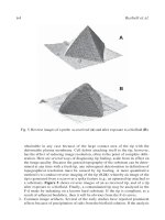
Fig. 2 . Typical AFM topography images of European brown human hairs: two untreated hairs: (A) hair 1, and (B) hair 2; and
two bleached hairs: (C) hair 1, and (D) hair 2. Examination of 10 images of each hair for both conditions suggests that the
bleached hairs appear to be more damaged than the untreated hairs.
98 Smith
2. Place the beaker in an ultrasonic bath and sonicate at room temperature for 30 s.
3. Pour away the detergent solution, rinse the hairs with copious amounts of double-
distilled water, and allow to air dry. Fibers can be subsequently stored between
filter papers.
4. Hair samples should be fixed to an AFM mounting assembly (nickel stub) using
double-sided carbon tape before AFM imaging.
3.2. AFM Imaging
1. The end of the cantilever should be placed over the center of the short axis of the
hair specimen.
2. The scan range should ideally be limited to an upper value of 20 µm. This obvi-
ates the scanner from exceeding its z range while tracking the curvature of hair
surfaces. Such artifacts have been reported elsewhere (4).
3. The resolution should be set to 500, that is, the topography dataset will comprise
500 lines × 500 pixels. A greater resolution can be used if desired.
4. An optimal scan rate of 3 Hz is recommended.
5. Surface architecture information is best revealed using a hypothetical light source
positioned to the left of the image.
6. Obtain an image of the hair surface and check the direction in which the cuticular
sheets overlap one another.
7. Change the scan direction so that the cuticular sheets overlap from left (root end)
to right (tip end; see Note 2).
8. Obtain 10 images each for treated and untreated regions for two hairs (4 × 10
images). Ideally, more hair fibers (approx 10) should be examined.
3.3. Image Analysis
1. Use the TopoMetrix Image analysis software (TopoMetrix SPM Lab. 1996, Ver-

sion 3.06.06, TopoMetrix Corporation, Santa Clara, CA) to load the saved topog-
raphy image and export the dataset as a text file. The images should not be
levelled and/or shaded before exporting the data. The cuticle step height program
requires the data to be delimited with comma separation and for the file header
information (first 18 rows of data) to be retained. The 40 text files should be
stored in a directory C:\subdirectory.
2. The text files should have three digit filenames. For example, “1b0.txt” refers to
hair 1 (the prefix), bleached (b, or u for untreated), first image (0). Image num-
bers range from 0 to 9.
3. Use the cuticle step height program, coded in Microsoft MS-DOS QuickBasic, to
calculate the cuticle step heights in all the images. A program listing is provided
in Subheading 3.4. (see Notes 3 and 4).
4. Four output text files, consisting of one long column of cuticle step heights in
nanometres (nm), are produced: hair 1, untreated; hair 1, treated (bleached); hair
2, untreated; and hair 2, treated.
5. The output text files can be read into a spreadsheet, such as Microsoft Excel, and
imported into a software package such as Microcal Origin 4.2 to produce line
Calculation of Cuticle Step Heights 99
graphs and histograms and to perform statistical analysis using, for example, one-
way analysis of variance (Fig. 3).
3.4. Cuticle Step Height Program Listing
REM**********************************************************************
REM*** IMAGE ANALYSIS OF ATOMIC FORCE MICROSCOPY IMAGES ***
REM*** OF HUMAN HAIR ***
REM*** ***
REM*** J.R. SMITH, SPM LABORATORY, ***
REM*** UNIVERSITY OF PORTSMOUTH ***
REM**********************************************************************
DIM height(1000): REM z-height at position 1 to 500
DIM deriv(1000): REM first derivative of height data

DIM maxgrad(1000): REM x-axis pixel position when deriv() >
gradient threshold
Fig. 3. Frequency histograms of cuticle step heights observed for bleach treated
(unshaded) and untreated (shaded) hairs. One-way analysis of variance showed there
to be no significant differences in the mean step heights for bleached and untreated
hairs (p <0.05, N
ន
10,000 steps per image).
100 Smith
DIM newstep(100): REM x-axis pixel position marking start of
each cuticle step
DIM endstep(100): REM x-axis pixel position marking end of each
cuticle step
DIM stepedge(100): REM calculated cuticle step height for output
sca = 20: REM scan range = 20 microns
res = 500: REM resolution = 500 pixels, image is 500 lines x 500
pixels
minh = 100: REM minimum height accepted as cuticle step
maxh = 900: REM maximum height accepted as cuticle step
numhair = 2: REM number of hairs to be examined
numtrt = 2: REM number of treatments to be examined (untreated &
bleached)
numimag = 10: REM number of AFM images per treatment, per hair
CLS
FOR hair = 1 TO numhair
FOR treat = 1 TO numtrt
IF treat = 1 THEN outname$ = RIGHT$(STR$(hair), 1) + “u”
ELSE outname$ = RIGHT$(STR$(hair), 1) + “b”
OPEN “C:\subdirectory\” + outname$ + “.txt” FOR OUTPUT AS
#2

FOR sample = 0 TO numimag-1
file$ = outname$ + RIGHT$(STR$(sample), 1)
OPEN “c:\subdirectory\” + file$ + “.txt” FOR INPUT AS #1
FOR n = 1 TO 18: REM reads superfluous header information
INPUT #1, x$
NEXT n
FOR major = 1 TO res: REM for ‘res’ lines of data
FOR n = 1 TO res: REM for ‘res’ columns of data
INPUT #1, height(n)
NEXT n
deriv(1) = 0
FOR n = 2 TO res
deriv(n) = height(n) - height(n-1)
NEXT n
num = 0: REM number of pixels positions where deriv() >
threshold, set to 10
FOR n = 1 TO res
check = ABS(deriv(n))
IF check > 10 THEN num = num+1: maxgrad(num) = n
NEXT n
count = 1
newstep(count) = maxgrad(count)
FOR n = 2 TO num
Calculation of Cuticle Step Heights 101
gap = maxgrad(n) - maxgrad(n-1)
IF gap >= 10 AND n >= 5 THEN count = count+1:
newstep(count) = maxgrad(n): endstep(count-1)
maxgrad(n-1)
NEXT n
endstep(count) = maxgrad(num)

FOR n = 1 TO count
height1 = newstep(n)
zheight1 = height(height1)
height2 = endstep(n)
zheight2 = height(zheight2)
stepedge(n) = INT(ABS(zheight1-zheight2))
NEXT n
FOR n = 1 TO count: REM removes step heights equal to
zero
IF stepedge(n) = 0 THEN count = count-1
NEXT n
FOR n = 1 TO count
IF stepedge(n) > minh AND stepedge(n) < maxh THEN
PRINT #2, stepedge(n): PRINT hair; treat; sample;
major; n; stepedge(n)
NEXT n
NEXT major
CLOSE #1
NEXT sample
CLOSE #2
NEXT treat
NEXT hair
END
4. Notes
1. Self-adhesive carbon discs (Agar Scientific, UK) tend to be more adhesive than
carbon tape, and are especially suited for wet-cell work (although the experi-
ments described here were performed in air).
2. The best way of viewing the surface architecture of cuticle scales is with the
orientation such that scales overlap from top–left (root end, highest point) to
bottom–right (tip end, lowest). With the TopoMetrix Discoverer TMX2000

instrument, this can be obtained by mounting the hair perpendicular to the long
axis of the cantilever and performing the scan at a scan rotation of either 90 or
270°, depending on juxtapositions of the root and tip ends. However, the required
orientation for the cuticle step height program is for the cuticle scales to overlap
from left to right. This can either be achieved by rotating the scan direction before
acquisition, or rotating the image, typically by about 20°, during the image-analy-
sis routine (Fig. 4). The latter, less favorable method reduces the scan range of
the image and so reduces the number of cuticle steps per image.
102 Smith
3. The program also assumes that the image is free from artefacts caused by the
scanner going off-range as a result of the gross curvature of the hair sample (see
Subheading 3.2., step 4). It is also necessary for the hair sample to be free from
endocuticular debris, which is sometimes observed at the foot of cuticle steps,
otherwise an erroneously low step height may be recorded.
4. The general program methodology is as follows: The program opens the input
text file and examines the first line consisting of 500 data points of height values
recorded in nanometres. The line of data is then derivatized using a first-order
algorithm to locate the positions of the cuticle steps on the x axis. Markers are set
that tag the start and end of each cuticle step on the line profile. This is achieved
by defining a threshold gradient, currently set to –10 nm/pixel. The minus sign
indicates that the cuticular sheets step down from left to right across the image;
the units are simply a result of z data being recorded in nanometers and lateral
information being recorded in pixels. The points where the derivative plot falls
below the threshold and subsequently rise above it mark the start and end of the
cuticle step, respectively. For this, the program considers all the points below the
threshold gradient and measures the gap between the current pixel position and
Fig. 4. The cuticle step height program requires the scales to overlap from left (root
end) to right (tip end). This can be achieved either by rotating the sample (preferred
method), or, as shown here, rotating the image (dataset) through 22°.
Calculation of Cuticle Step Heights 103

its previous value. If the gap is greater than a given clearance, currently set to 10
pixels (0.4 µm for a resolution of 500 pixels), then a new cuticle has been identi-
fied. The routine continues until the end of the line. Cuticle step heights are then
calculated by measuring the vertical distance between the start and end markers
for each cuticle step. Steps heights less than 100 nm or greater than 900 nm are
neglected. The process is repeated for the remaining 499 lines of the input text
file. The program can easily be adapted to open further text files corresponding
to more hair images to construct a more representative sample set.
Acknowledgments
Thanks are owed to the Royal Society of Chemistry and Royal Society for
financial support.
References
1. Goddard, E. D. and Schmitt, R. L. (1994) Atomic force microscopy investigations
into the absorption of cationic polymers. Cosmet. Toiletr. 109, 55–61.
2. Schmitt, R. L. and Goddard, E. D. (1994) Atomic force microscopy. II. Investiga-
tion into the absorption of cationic polymers. Cosmet. Toilet. 109(12), 83–93.
3. O’Connor, S. D., Komisarek, K. L. and Baldeschwielder, J. D. (1995) Atomic
force microscopy of human hair cuticles: A microscopic study of environmental
effects on hair morphology. J. Invest. Dermatol. 105, 96–99.
4. Hössel, P., Sander, D. I. R., and Schrepp, W. (1996) Scanning force microscopy.
Cosmet. Toilet.111, 57–65.
5. You, H. and Yu, L. (1997) Atomic force microscopy as a tool for study of human
hair. Scanning 19, 431–437.
6. Smith, J. R. (1998) A quantitative method for analysing AFM images of the outer
surfaces of human hair. J. Microsc. 191, 223–228.
7. Smith, J. R., Connell, S. D., and Swift, J. A. (1999) Stereoscopic display of atomic
force microscope images using anaglyph techniques. J. Microsc. 196, 347–351.
8. Swift, J. A. and Smith, J. R. (2000) Atomic force microscopy of human hair.
Scanning 22, 310–318.
9. Swift, J. A. and Smith, J. R. (2000) Surface striations of human hair and other

mammalian keratin fibres. Proc. 10th Int. Wool Text. Res. Conf., Aachen, Ger-
many, 26 Nov to 1 Dec 2000, HH-2, 1–9. ISBN 3–00–007905-X.
10. Swift, J. A. and Smith, J. R. (2001) Microscopic investigations on the epicuticle
of mammalian keratin fibres. J. Microsc. 204, 203–211.
11. Smith, J. R. and Swift, J. A. (2002) Lamellar sub-components of the cuticular cell
membrane complex of mammalian keratin fibres show friction and hardness con-
trast by AFM. J. Microsc. 206, 182–193.
12. Hashimoto and Shibazaki, 1976; Hashimoto, K. and Shibazaki, S. (1976) Ultra-
structural study on differentiation and function of hair, in Biology and Disease of
the Hair (Kobori, T. and Montagna, W. eds.), University Park Press Baltimore,
pp. 23–57.