A HEAT TRANSFER TEXTBOOK - THIRD EDITION Episode 1 Part 6 ppt

114 Heat exchanger design §3.2
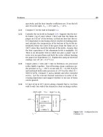
Figure 3.11 A typical case of a heat exchanger in which U
varies dramatically.
The second limitation—our use of a constant value of U— is more
serious. The value of U must be negligibly dependent on T to complete
the integration of eqn. (3.7). Even if U ≠ fn(T ), the changing flow con-
figuration and the variation of temperature can still give rise to serious
variations of U within a given heat exchanger. Figure 3.11 shows a typ-
ical situation in which the variation of U within a heat exchanger might
be great. In this case, the mechanism of heat exchange on the water side
is completely altered when the liquid is finally boiled away. If U were
uniform in each portion of the heat exchanger, then we could treat it as
two different exchangers in series.
However, the more common difficulty that we face is that of design-
ing heat exchangers in which U varies continuously with position within
it. This problem is most severe in large industrial shell-and-tube config-
urations
1
(see, e.g., Fig. 3.5 or Fig. 3.12) and less serious in compact heat
exchangers with less surface area. If U depends on the location, analyses
such as we have just completed [eqn. (3.1) to eqn. (3.13)] must be done
using an average U defined as

A
0
UdA/A.
1
Actual heat exchangers can have areas well in excess of 10,000 m
2
. Large power
plant condensers and other large exchangers are often remarkably big pieces of equip-

ment.
Figure 3.12 The heat exchange surface for a steam genera-
tor. This PFT-type integral-furnace boiler, with a surface area
of 4560 m
2
, is not particularly large. About 88% of the area
is in the furnace tubing and 12% is in the boiler (Photograph
courtesy of Babcock and Wilcox Co.)
115
116 Heat exchanger design §3.2
LMTD correction factor, F. Suppose that we have a heat exchanger in
which U can reasonably be taken constant, but one that involves such
configurational complications as multiple passes and/or cross-flow. In
such cases it is necessary to rederive the appropriate mean temperature
difference in the same way as we derived the LMTD. Each configuration
must be analyzed separately and the results are generally more compli-
cated than eqn. (3.13).
This task was undertaken on an ad hoc basis during the early twen-
tieth century. In 1940, Bowman, Mueller and Nagle [3.2] organized such
calculations for the common range of heat exchanger configurations. In
each case they wrote
Q = UA(LMTD) ·F






T
t

out
−T
t
in
T
s
in
−T
t
in
  
P
,
T
s
in
−T
s
out
T
t
out
−T
t
in
  
R







(3.14)
where T
t
and T
s
are temperatures of tube and shell flows, respectively.
The factor F is an LMTD correction that varies from unity to zero, depend-
ing on conditions. The dimensionless groups P and R have the following
physical significance:
• P is the relative influence of the overall temperature difference
(T
s
in
− T
t
in
) on the tube flow temperature. It must obviously be
less than unity.
• R, according to eqn. (3.10), equals the heat capacity ratio C
t
/C
s
.
• If one flow remains at constant temperature (as, for example, in
Fig. 3.9), then either P or R will equal zero. In this case the simple
LMTD will be the correct ∆T
mean

and F must go to unity.
The factor F is defined in such a way that the LMTD should always be
calculated for the equivalent counterflow single-pass exchanger with the
same hot and cold temperatures. This is explained in Fig. 3.13.
Bowman et al. [3.2] summarized all the equations for F, in various con-
figurations, that had been dervied by 1940. They presented them graphi-
cally in not-very-accurate figures that have been widely copied. The TEMA
[3.1] version of these curves has been recalculated for shell-and-tube heat
exchangers, and it is more accurate. We include two of these curves in
Fig. 3.14(a) and Fig. 3.14(b). TEMA presents many additional curves for
more complex shell-and-tube configurations. Figures 3.14(c) and 3.14(d)
§3.2 Evaluation of the mean temperature difference in a heat exchanger 117
Figure 3.13 The basis of the LMTD in a multipass exchanger,
prior to correction.
are the Bowman et al. curves for the simplest cross-flow configurations.
Gardner and Taborek [3.3] redeveloped Fig. 3.14(c) over a different range
of parameters. They also showed how Fig. 3.14(a) and Fig. 3.14(b) must
be modified if the number of baffles in a tube-in-shell heat exchanger is
large enough to make it behave like a series of cross-flow exchangers.
We have simplified Figs. 3.14(a) through 3.14(d) by including curves
only for R1. Shamsundar [3.4] noted that for R>1, one may obtain F
using a simple reciprocal rule. He showed that so long as a heat exchan-
ger has a uniform heat transfer coefficient and the fluid properties are
constant,
F(P,R) = F(PR,1/R) (3.15)
Thus, if R is greater than unity, one need only evaluate F using PR in
place of P and 1/R in place of R.
Example 3.4
5.795 kg/s of oil flows through the shell side of a two-shell pass, four-
a. F for a one-shell-pass, four, six-, tube-pass exchanger.

b. F for a two-shell-pass, four or more tube-pass exchanger.
Figure 3.14 LMTD correction factors, F, for multipass shell-
and-tube heat exchangers and one-pass cross-flow exchangers.
118
c. F for a one-pass cross-flow exchanger with both passes unmixed.
d. F for a one-pass cross-flow exchanger with one pass mixed.
Figure 3.14 LMTD correction factors, F, for multipass shell-
and-tube heat exchangers and one-pass cross-flow exchangers.
119
120 Heat exchanger design §3.3
tube-pass oil cooler. The oil enters at 181
◦
C and leaves at 38
◦
C. Water
flows in the tubes, entering at 32
◦
C and leaving at 49
◦
C. In addition,
c
p
oil
= 2282 J/kg·K and U = 416 W/m
2
K. Find how much area the
heat exchanger must have.
Solution.
LMTD =
(T

h
in
−T
c
out
) −(T
h
out
−T
c
in
)
ln

T
h
in
−T
c
out
T
h
out
−T
c
in

=
(181 −49) −(38 −32)
ln


181 −49
38 −32

= 40.76 K
R =
181 −38
49 −32
= 8.412 P =
49 −32
181 −32
= 0.114
Since R>1, we enter Fig. 3.14(b) using P = 8.412(0.114) = 0.959 and
R = 1/8.412 = 0.119 and obtain F = 0.92.
2
It follows that:
Q = UAF(LMTD)
5.795(2282)(181 −38) = 416(A)(0.92)(40.76)
A = 121.2m
2
3.3 Heat exchanger effectiveness
We are now in a position to predict the performance of an exchanger once
we know its configuration and the imposed differences. Unfortunately,
we do not often know that much about a system before the design is
complete.
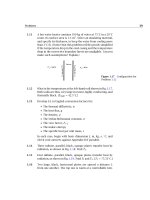
Often we begin with information such as is shown in Fig. 3.15.If
we sought to calculate Q in such a case, we would have to do so by
guessing an exit temperature such as to make Q
h
= Q

c
= C
h
∆T
h
=
C
c
∆T
c
. Then we could calculate Q from UA(LMTD) or UAF (LMTD) and
check it against Q
h
. The answers would differ, so we would have to guess
new exit temperatures and try again.
Such problems can be greatly simplified with the help of the so-called
effectiveness-NTU method. This method was first developed in full detail
2
Notice that, for a 1 shell-pass exchanger, these R and P lines do not quite intersect
[see Fig. 3.14(a)]. Therefore, one could not obtain these temperatures with any single-
shell exchanger.
§3.3 Heat exchanger effectiveness 121
Figure 3.15 A design problem in which the LMTD cannot be
calculated a priori.
by Kays and London [3.5] in 1955, in a book titled Compact Heat Exchang-
ers. We should take particular note of the title. It is with compact heat
exchangers that the present method can reasonably be used, since the
overall heat transfer coefficient is far more likely to remain fairly uni-
form.
The heat exchanger effectiveness is defined as

ε ≡
C
h
(T
h
in
−T
h
out
)
C
min
(T
h
in
−T
c
in
)
=
C
c
(T
c
out
−T
c
in
)
C

min
(T
h
in
−T
c
in
)
(3.16)
where C
min
is the smaller of C
c
and C
h
. The effectiveness can be inter-
preted as
ε =
actual heat transferred
maximum heat that could possibly be
transferred from one stream to the other
It follows that
Q = εC
min
(T
h
in
−T
c
in

) (3.17)
A second definition that we will need was originally made by E.K.W.
Nusselt, whom we meet again in Part III. This is the number of transfer
units (NTU):
NTU ≡
UA
C
min
(3.18)
122 Heat exchanger design §3.3
This dimensionless group can be viewed as a comparison of the heat
capacity of the heat exchanger, expressed in W/K, with the heat capacity
of the flow.
We can immediately reduce the parallel-flow result from eqn. (3.9)to
the following equation, based on these definitions:
−

C
min
C
c
+
C
min
C
h

NTU = ln

−


1 +
C
c
C
h

ε
C
min
C
c
+1

(3.19)
We solve this for ε and, regardless of whether C
min
is associated with the
hot or cold flow, obtain for the parallel single-pass heat exchanger:
ε ≡
1 −exp
[
−(1 +C
min
/C
max
)NTU
]
1 +C
min

/C
max
= fn

C
min
C
max
, NTU only

(3.20)
The corresponding expression for the counterflow case is
ε =
1 −exp
[
−(1 −C
min
/C
max
)NTU
]
1 −(C
min
/C
max
) exp[−(1 − C
min
/C
max
)NTU]

(3.21)
Equations (3.20) and (3.21) are given in graphical form in Fig. 3.16.
Similar calculations give the effectiveness for the other heat exchanger
configurations (see [3.5] and Problem 3.38), and we include some of the
resulting effectiveness plots in Fig. 3.17. To see how the effectiveness
can conveniently be used to complete a design, consider the following
two examples.
Example 3.5
Consider the following parallel-flow heat exchanger specification:
cold flow enters at 40
◦
C: C
c
= 20, 000 W/K
hot flow enters at 150
◦
C: C
h
= 10, 000 W/K
A = 30 m
2
U = 500 W/m
2
K.
Determine the heat transfer and the exit temperatures.
Solution. In this case we do not know the exit temperatures, so it
is not possible to calculate the LMTD. Instead, we can go either to the
parallel-flow effectiveness chart in Fig. 3.16 or to eqn. (3.20), using
NTU =
UA

C
min
=
500(30)
10, 000
= 1.5
C
min
C
max
= 0.5
§3.3 Heat exchanger effectiveness 123
Figure 3.16 The effectiveness of parallel and counterflow heat
exchangers. (Data provided by A.D. Krauss.)
and we obtain ε = 0.596. Now from eqn. (3.17), we find that
Q = εC
min
(T
h
in
−T
c
in
) = 0.596(10, 000)(110)
= 655, 600 W = 655.6kW
Finally, from energy balances such as are expressed in eqn. (3.4), we
get
T
h
out

= T
h
in
−
Q
C
h
= 150 −
655, 600
10, 000
= 84.44
◦
C
T
c
out
= T
c
in
+
Q
C
c
= 40 +
655, 600
20, 000
= 72.78
◦
C
Example 3.6

Suppose that we had the same kind of exchanger as we considered
in Example 3.5, but that the area remained unspecified as a design
variable. Then calculate the area that would bring the hot flow out at
90
◦
C.
Solution. Once the exit cold fluid temperature is known, the prob-
lem can be solved with equal ease by either the LMTD or the effective-
Figure 3.17 The effectiveness of some other heat exchanger
configurations. (Data provided by A.D. Krauss.)
124
§3.3 Heat exchanger effectiveness 125
ness approach.
T
c
out
= T
c
in
+
C
h
C
c
(T
h
in
−T
h
out

) = 40 +
1
2
(150 −90) = 70
◦
C
Then, using the effectiveness method,
ε =
C
h
(T
h
in
−T
h
out
)
C
min
(T
h
in
−T
c
in
)
=
10, 000(150 − 90)
10, 000(150 − 40)
= 0.5455

so from Fig. 3.16 we read NTU 1.15 = UA/C
min
. Thus
A =
10, 000(1.15)
500
= 23.00 m
2
We could also have calculated the LMTD:
LMTD =
(150 −40) −(90 −70)
ln(110/20)
= 52.79 K
so from Q = UA(LMTD), we obtain
A =
10, 000(150 − 90)
500(52.79)
= 22.73 m
2
The answers differ by 1%, which reflects graph reading inaccuracy.
When the temperature of either fluid in a heat exchanger is uniform,
the problem of analyzing heat transfer is greatly simplified. We have
already noted that no F-correction is needed to adjust the LMTD in this
case. The reason is that when only one fluid changes in temperature, the
configuration of the exchanger becomes irrelevant. Any such exchanger
is equivalent to a single fluid stream flowing through an isothermal pipe.
3
Since all heat exchangers are equivalent in this case, it follows that
the equation for the effectiveness in any configuration must reduce to
the same common expression as C

max
approaches infinity. The volumet-
ric heat capacity rate might approach infinity because the flow rate or
specific heat is very large, or it might be infinite because the flow is ab-
sorbing or giving up latent heat (as in Fig. 3.9). The limiting effectiveness
expression can also be derived directly from energy-balance considera-
tions (see Problem 3.11), but we obtain it here by letting C
max
→∞in
either eqn. (3.20) or eqn. (3.21). The result is
lim
C
max
→∞
ε = 1 − e
−NTU
(3.22)
3
We make use of this notion in Section 7.4, when we analyze heat convection in pipes
and tubes.
126 Heat exchanger design §3.4
Eqn. (3.22) defines the curve for C
min
/C
max
= 0 in all six of the effective-
ness graphs in Fig. 3.16 and Fig. 3.17.
3.4 Heat exchanger design
The preceding sections provided means for designing heat exchangers
that generally work well in the design of smaller exchangers—typically,

the kind of compact cross-flow exchanger used in transportation equip-
ment. Larger shell-and-tube exchangers pose two kinds of difficulty in
relation to U. The first is the variation of U through the exchanger, which
we have already discussed. The second difficulty is that convective heat
transfer coefficients are very hard to predict for the complicated flows
that move through a baffled shell.
We shall achieve considerable success in using analysis to predict
h’s
for various convective flows in Part III. The determination of
h in a baffled
shell remains a problem that cannot be solved analytically. Instead, it
is normally computed with the help of empirical correlations or with
the aid of large commercial computer programs that include relevant
experimental correlations. The problem of predicting
h when the flow is
boiling or condensing is even more complicated. A great deal of research
is at present aimed at perfecting such empirical predictions.
Apart from predicting heat transfer, a host of additional considera-
tions must be addressed in designing heat exchangers. The primary ones
are the minimization of pumping power and the minimization of fixed
costs.
The pumping power calculation, which we do not treat here in any
detail, is based on the principles discussed in a first course on fluid me-
chanics. It generally takes the following form for each stream of fluid
through the heat exchanger:
pumping power =

˙
m
kg

s


∆p
ρ
N/m
2
kg/m
3

=
˙
m∆p
ρ

N·m
s

=
˙
m∆p
ρ
(W)
(3.23)
where
˙
m is the mass flow rate of the stream, ∆p the pressure drop of
the stream as it passes through the exchanger, and ρ the fluid density.
Determining the pressure drop can be relatively straightforward in a
single-pass pipe-in-tube heat exchanger or extremely difficulty in, say, a

§3.4 Heat exchanger design 127
shell-and-tube exchanger. The pressure drop in a straight run of pipe,
for example, is given by
∆p = f

L
D
h

ρu
2
av
2
(3.24)
where L is the length of pipe, D
h
is the hydraulic diameter, u
av
is the
mean velocity of the flow in the pipe, and f is the Darcy-Weisbach friction
factor (see Fig. 7.6).
Optimizing the design of an exchanger is not just a matter of making
∆p as small as possible. Often, heat exchange can be augmented by em-
ploying fins or roughening elements in an exchanger. (We discuss such
elements in Chapter 4; see, e.g., Fig. 4.6). Such augmentation will invari-
ably increase the pressure drop, but it can also reduce the fixed cost of
an exchanger by increasing U and reducing the required area. Further-
more, it can reduce the required flow rate of, say, coolant, by increasing
the effectiveness and thus balance the increase of ∆p in eqn. (3.23).
To better understand the course of the design process, faced with

such an array of trade-offs of advantages and penalties, we follow Ta-
borek’s [3.6] list of design considerations for a large shell-and-tube ex-
changer:
• Decide which fluid should flow on the shell side and which should
flow in the tubes. Normally, this decision will be made to minimize
the pumping cost. If, for example, water is being used to cool oil,
the more viscous oil would flow in the shell. Corrosion behavior,
fouling, and the problems of cleaning fouled tubes also weigh heav-
ily in this decision.
• Early in the process, the designer should assess the cost of the cal-
culation in comparison with:
(a) The converging accuracy of computation.
(b) The investment in the exchanger.
(c) The cost of miscalculation.
• Make a rough estimate of the size of the heat exchanger using, for
example, U values from Table 2.2 and/or anything else that might
be known from experience. This serves to circumscribe the sub-
sequent trial-and-error calculations; it will help to size flow rates
and to anticipate temperature variations; and it will help to avoid
subsequent errors.
128 Heat exchanger design §3.4
• Evaluate the heat transfer, pressure drop, and cost of various ex-
changer configurations that appear reasonable for the application.
This is usually done with large-scale computer programs that have
been developed and are constantly being improved as new research
is included in them.
The computer runs suggested by this procedure are normally very com-
plicated and might typically involve 200 successive redesigns, even when
relatively efficient procedures are used.
However, most students of heat transfer will not have to deal with

such designs. Many, if not most, will be called upon at one time or an-
other to design smaller exchangers in the range 0.1 to 10 m
2
. The heat
transfer calculation can usually be done effectively with the methods de-
scribed in this chapter. Some useful sources of guidance in the pressure
drop calculation are the Heat Exchanger Design Handbook [3.7], the data
in Idelchik’s collection [3.8], the TEMA design book [3.1], and some of the
other references at the end of this chapter.
In such a calculation, we start off with one fluid to heat and one to
cool. Perhaps we know the flow heat capacity rates (C
c
and C
h
), certain
temperatures, and/or the amount of heat that is to be transferred. The
problem can be annoyingly wide open, and nothing can be done until it is
somehow delimited. The normal starting point is the specification of an
exchanger configuration, and to make this choice one needs experience.
The descriptions in this chapter provide a kind of first level of experi-
ence. References [3.5, 3.7, 3.9, 3.10, 3.11, 3.12] provide a second level.
Manufacturer’s catalogues are an excellent source of more advanced in-
formation.
Once the exchanger configuration is set, U will be approximately set
and the area becomes the basic design variable. The design can then
proceed along the lines of Section 3.2 or 3.3. If it is possible to begin
with a complete specification of inlet and outlet temperatures,
Q

C∆T

= U

known
AF(LMTD)

 
calculable
Then A can be calculated and the design completed. Usually, a reevalu-
ation of U and some iteration of the calculation is needed.
More often, we begin without full knowledge of the outlet tempera-
tures. In such cases, we normally have to invent an appropriate trial-and-
error method to get the area and a more complicated sequence of trials if
we seek to optimize pressure drop and cost by varying the configuration
Problems 129
as well. If the C’s are design variables, the U will change significantly,
because
h’s are generally velocity-dependent and more iteration will be
needed.
We conclude Part I of this book facing a variety of incomplete issues.
Most notably, we face a serious need to be able to determine convective
heat transfer coefficients. The prediction of
h depends on a knowledge of
heat conduction. We therefore turn, in Part II, to a much more thorough
study of heat conduction analysis than was undertaken in Chapter 2.
In addition to setting up the methodology ultimately needed to predict
h’s, Part II will also deal with many other issues that have great practical
importance in their own right.
Problems
3.1 Can you have a cross-flow exchanger in which both flows are
mixed? Discuss.

3.2 Find the appropriate mean radius,
r , that will make
Q = kA(
r)∆T /(r
o
−r
i
), valid for the one-dimensional heat con-
duction through a thick spherical shell, where A(
r) = 4πr
2
(cf.
Example 3.1).
3.3 Rework Problem 2.14, using the methods of Chapter 3.
3.4 2.4 kg/s of a fluid have a specific heat of 0.81 kJ/kg·K enter a
counterflow heat exchanger at 0
◦
C and are heated to 400
◦
Cby
2 kg/s of a fluid having a specific heat of 0.96 kJ/kg·K entering
the unit at 700
◦
C. Show that to heat the cooler fluid to 500
◦
C,
all other conditions remaining unchanged, would require the
surface area for a heat transfer to be increased by 87.5%.
3.5 A cross-flow heat exchanger with both fluids unmixed is used
to heat water (c

p
= 4.18 kJ/kg·K) from 40
◦
Cto80
◦
C, flowing at
the rate of 1.0 kg/s. What is the overall heat transfer coefficient
if hot engine oil (c
p
= 1.9 kJ/kg·K), flowing at the rate of 2.6
kg/s, enters at 100
◦
C? The heat transfer area is 20 m
2
. (Note
that you can use either an effectiveness or an LMTD method.
It would be wise to use both as a check.)
3.6 Saturated non-oil-bearing steam at 1 atm enters the shell pass
of a two-tube-pass shell condenser with thirty 20 ft tubes in
130 Chapter 3: Heat exchanger design
each tube pass. They are made of schedule 160, ¾ in. steel
pipe (nominal diameter). A volume flow rate of 0.01 ft
3
/s of
water entering at 60
◦
F enters each tube. The condensing heat
transfer coefficient is 2000 Btu/h·ft
2
·

◦
F, and we calculate h =
1380 Btu/h·ft
2
·
◦
F for the water in the tubes. Estimate the exit
temperature of the water and mass rate of condensate [
˙
m
c

8393 lb
m
/h.]
3.7 Consider a counterflow heat exchanger that must cool 3000
kg/h of mercury from 150
◦
Fto128
◦
F. The coolant is 100 kg/h
of water, supplied at 70
◦
F. If U is 300 W/m
2
K, complete the
design by determining reasonable value for the area and the
exit-water temperature. [A = 0.147 m
2
.]

3.8 An automobile air-conditioner gives up 18 kW at 65 km/h if the
outside temperature is 35
◦
C. The refrigerant temperature is
constant at 65
◦
C under these conditions, and the air rises 6
◦
C
in temperature as it flows across the heat exchanger tubes. The
heat exchanger is of the finned-tube type shown in Fig. 3.6b,
with U  200 W/m
2
K. If U ∼ (air velocity)
0.7
and the mass flow
rate increases directly with the velocity, plot the percentage
reduction of heat transfer in the condenser as a function of air
velocity between 15 and 65 km/h.
3.9 Derive eqn. (3.21).
3.10 Derive the infinite NTU limit of the effectiveness of parallel and
counterflow heat exchangers at several values of C
min
/C
max
.
Use common sense and the First Law of Thermodynamics, and
refer to eqn. (3.2) and eqn. (3.21) only to check your results.
3.11 Derive the equation ε = (NTU,C
min

/C
max
) for the heat exchan-
ger depicted in Fig. 3.9.
3.12 A single-pass heat exchanger condenses steam at 1 atm on
the shell side and heats water from 10
◦
Cto30
◦
C on the tube
side with U = 2500 W/m
2
K. The tubing is thin-walled, 5 cm in
diameter, and2minlength. (a) Your boss asks whether the
exchanger should be counterflow or parallel-flow. How do you
advise her? Evaluate: (b) the LMTD; (c)
˙
m
H
2
O
; (d) ε.[ε 0.222.]
Problems 131
3.13 Air at 2 kg/s and 27
◦
C and a stream of water at 1.5 kg/s and
60
◦
C each enter a heat exchanger. Evaluate the exit tempera-
tures if A =12m

2
, U = 185 W/m
2
K, and:
a. The exchanger is parallel flow;
b. The exchanger is counterflow [T
h
out
 54.0
◦
C.];
c. The exchanger is cross-flow, one stream mixed;
d. The exchanger is cross-flow, neither stream mixed.
[T
h
out
= 53.62
◦
C.]
3.14 Air at 0.25 kg/s and 0
◦
C enters a cross-flow heat exchanger.
It is to be warmed to 20
◦
C by 0.14 kg/s of air at 50
◦
C. The
streams are unmixed. As a first step in the design process,
plot U against A and identify the approximate range of area
for the exchanger.

3.15 A particular two shell-pass, four tube-pass heat exchanger uses
20 kg/s of river water at 10
◦
C on the shell side to cool 8 kg/s
of processed water from 80
◦
Cto25
◦
C on the tube side. At
what temperature will the coolant be returned to the river? If
U is 800 W/m
2
K, how large must the exchanger be?
3.16 A particular cross-flow process heat exchanger operates with
the fluid mixed on one side only. When it is new, U = 2000
W/m
2
K, T
c
in
=25
◦
C, T
c
out
=80
◦
C, T
h
in

= 160
◦
C, and T
h
out
=
70
◦
C. After 6 months of operation, the plant manager reports
that the hot fluid is only being cooled to 90
◦
C and that he is
suffering a 30% reduction in total heat transfer. What is the
fouling resistance after 6 months of use? (Assume no reduc-
tion of cold-side flow rate by fouling.)
3.17 Water at 15
◦
C is supplied to a one-shell-pass, two-tube-pass
heat exchanger to cool 10 kg/s of liquid ammonia from 120
◦
C
to 40
◦
C. You anticipate a U on the order of 1500 W/m
2
K when
the water flows in the tubes. If A is to be 90 m
2
, choose the
correct flow rate of water.

3.18 Suppose that the heat exchanger in Example 3.5 had been a two
shell-pass, four tube-pass exchanger with the hot fluid moving
in the tubes. (a) What would be the exit temperature in this
case? [T
c
out
= 75.09
◦
C.] (b) What would be the area if we wanted
132 Chapter 3: Heat exchanger design
the hot fluid to leave at the same temperature that it does in
the example?
3.19 Plot the maximum tolerable fouling resistance as a function
of U
new
for a counterflow exchanger, with given inlet temper-
atures, if a 30% reduction in U is the maximum that can be
tolerated.
3.20 Water at 0.8 kg/s enters the tubes of a two-shell-pass, four-
tube-pass heat exchanger at 17
◦
C and leaves at 37
◦
C. It cools
0.5 kg/s of air entering the shell at 250
◦
C with U = 432 W/m
2
K.
Determine: (a) the exit air temperature; (b) the area of the heat

exchanger; and (c) the exit temperature if, after some time,
the tubes become fouled with R
f
= 0.0005 m
2
K/W. [(c) T
air
out
= 140.5
◦
C.]
3.21 You must cool 78 kg/min of a 60%-by-mass mixture of glycerin
in water from 108
◦
Cto50
◦
C using cooling water available at
7
◦
C. Design a one-shell-pass, two-tube-pass heat exchanger if
U = 637 W/m
2
K. Explain any design decision you make and
report the area, T
H
2
O
out
, and any other relevant features.
3.22 A mixture of 40%-by-weight glycerin, 60% water, enters a smooth

0.113 m I.D. tube at 30
◦
C. The tube is kept at 50
◦
C, and
˙
m
mixture
= 8 kg/s. The heat transfer coefficient inside the pipe is 1600
W/m
2
K. Plot the liquid temperature as a function of position
in the pipe.
3.23 Explain in physical terms why all effectiveness curves Fig. 3.16
and Fig. 3.17 have the same slope as NTU → 0. Obtain this
slope from eqns. (3.20) and (3.21).
3.24 You want to cool air from 150
◦
Cto60
◦
C but you cannot af-
ford a custom-built heat exchanger. You find a used cross-flow
exchanger (both fluids unmixed) in storage. It was previously
used to cool 136 kg/min of NH
3
vapor from 200
◦
C to 100
◦
C us-

ing 320 kg/min of water at 7
◦
C; U was previously 480 W/m
2
K.
How much air can you cool with this exchanger, using the same
water supply, if U is approximately unchanged? (Actually, you
would have to modify U using the methods of Chapters 6 and
7 once you had the new air flow rate, but that is beyond our
present scope.)
Problems 133
3.25 A one tube-pass, one shell-pass, parallel-flow, process heat ex-
changer cools 5 kg/s of gaseous ammonia entering the shell
side at 250
◦
C and boils 4.8 kg/s of water in the tubes. The wa-
ter enters subcooled at 27
◦
C and boils when it reaches 100
◦
C.
U = 480 W/m
2
K before boiling begins and 964 W/m
2
K there-
after. The area of the exchanger is 45 m
2
, and h
fg

for water
is 2.257 ×10
6
J/kg. Determine the quality of the water at the
exit.
3.26 0.72 kg/s of superheated steam enters a crossflow heat ex-
changer at 240
◦
C and leaves at 120
◦
C. It heats 0.6 kg/s of water
entering at 17
◦
C. U = 612 W/m
2
K. By what percentage will the
area differ if a both-fluids-unmixed exchanger is used instead
of a one-fluid-unmixed exchanger? [−1.8%]
3.27 Compare values of F from Fig. 3.14(c) and Fig. 3.14(d) for the
same conditions of inlet and outlet temperatures. Is the one
with the higher F automatically the more desirable exchanger?
Discuss.
3.28 Compare values of ε for the same NTU and C
min
/C
max
in paral-
lel and counterflow heat exchangers. Is the one with the higher
ε automatically the more desirable exchanger? Discuss.
3.29 The irreversibility rate of a process is equal to the rate of en-

tropy production times the lowest absolute sink temperature
accessible to the process. Calculate the irreversibility (or lost
work) for the heat exchanger in Example 3.4. What kind of
configuration would reduce the irreversibility, given the same
end temperatures.
3.30 Plot T
oil
and T
H
2
O
as a function of position in a very long coun-
terflow heat exchanger where water enters at 0
◦
C, with C
H
2
O
=
460 W/K, and oil enters at 90
◦
C, with C
oil
= 920 W/K, U = 742
W/m
2
K, and A =10m
2
. Criticize the design.
3.31 Liquid ammonia at 2 kg/s is cooled from 100

◦
Cto30
◦
C in the
shell side of a two shell-pass, four tube-pass heat exchanger
by 3 kg/s of water at 10
◦
C. When the exchanger is new, U =
750 W/m
2
K. Plot the exit ammonia temperature as a function
of the increasing tube fouling factor.
134 Chapter 3: Heat exchanger design
3.32 A one shell-pass, two tube-pass heat exchanger cools 0.403
kg/s of methanol from 47
◦
Cto7
◦
C on the shell side. The
coolant is 2.2 kg/s of Freon 12, entering the tubes at −33
◦
C,
with U = 538 W/m
2
K. A colleague suggests that this arrange-
ment wastes Freon. She thinks you could do almost as well if
you cut the Freon flow rate all the way down to 0.8 kg/s. Cal-
culate the new methanol outlet temperature that would result
from this flow rate, and evaluate her suggestion.
3.33 The factors dictating the heat transfer coefficients in a certain

two shell-pass, four tube-pass heat exchanger are such that
U increases as (
˙
m
shell
)
0.6
. The exchanger cools 2 kg/s of air
from 200
◦
Cto40
◦
C using 4.4 kg/s of water at 7
◦
C, and U = 312
W/m
2
K under these circumstances. If we double the air flow,
what will its temperature be leaving the exchanger? [T
air
out
=
61
◦
C.]
3.34 A flow rate of 1.4 kg/s of water enters the tubes of a two-shell-
pass, four-tube-pass heat exchanger at 7
◦
C. A flow rate of 0.6
kg/s of liquid ammonia at 100

◦
C is to be cooled to 30
◦
Con
the shell side; U = 573 W/m
2
K. (a) How large must the heat
exchanger be? (b) How large must it be if, after some months,
a fouling factor of 0.0015 will build up in the tubes, and we still
want to deliver ammonia at 30
◦
C? (c) If we make it large enough
to accommodate fouling, to what temperature will it cool the
ammonia when it is new? (d) At what temperature does water
leave the new, enlarged exchanger? [(d) T
H
2
O
= 49.9
◦
C.]
3.35 Both C’s in a parallel-flow heat exchanger are equal to 156 W/K,
U = 327 W/m
2
K and A = 2m
2
. The hot fluid enters at 140
◦
C
and leaves at 90

◦
C. The cold fluid enters at 40
◦
C. If both C’s
are halved, what will be the exit temperature of the hot fluid?
3.36 A 1.68 ft
2
cross-flow heat exchanger with one fluid mixed con-
denses steam at atmospheric pressure (
h = 2000 Btu/h·ft
2
·
◦
F)
and boils methanol (T
sat
= 170
◦
F and h = 1500 Btu/h·ft
2
·
◦
F) on
the other side. Evaluate U (neglecting resistance of the metal),
LMTD, F, NTU, ε, and Q.
3.37 Eqn. (3.21) is troublesome when C
min
/C
max
= 1. Develop a

working equation for ε in this case. Compare it with Fig. 3.16.
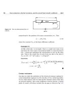
136 Chapter 3: Heat exchanger design
c. Determine the air temperature at the point where the lead
has just finished solidifying.
d. Determine the height that the tower must have in order to
function as desired. The heat transfer coefficient between
the air and the droplets is
h = 318 W/m
2
K.
References
[3.1] Tubular Exchanger Manufacturer’s Association. Standards of
Tubular Exchanger Manufacturer’s Association. New York, 4th and
6th edition, 1959 and 1978.
[3.2] R. A. Bowman, A. C. Mueller, and W. M. Nagle. Mean temperature
difference in design. Trans. ASME, 62:283–294, 1940.
[3.3] K. Gardner and J. Taborek. Mean temperature difference: A reap-
praisal. AIChE J., 23(6):770–786, 1977.
[3.4] N. Shamsundar. A property of the log-mean temperature-
difference correction factor. Mechanical Engineering News, 19(3):
14–15, 1982.
[3.5] W. M. Kays and A. L. London. Compact Heat Exchangers. McGraw-
Hill Book Company, New York, 3rd edition, 1984.
[3.6] J. Taborek. Evolution of heat exchanger design techniques. Heat
Transfer Engineering, 1(1):15–29, 1979.
[3.7] G. F. Hewitt, editor. Heat Exchanger Design Handbook 1998. Begell
House, New York, 1998.
[3.8] E. Fried and I.E. Idelchik. Flow Resistance: A Design Guide for En-
gineers. Hemisphere Publishing Corp., New York, 1989.
[3.9] R. H. Perry, D. W. Green, and J. Q. Maloney, editors. Perry’s Chem-

ical Engineers’ Handbook. McGraw-Hill Book Company, New York,
7th edition, 1997.
[3.10] D. M. Considine. Energy Technology Handbook. McGraw-Hill Book
Company, New York, 1975.
[3.11] A. P. Fraas. Heat Exchanger Design. John Wiley & Sons, Inc., New
York, 2nd edition, 1989.
References 137
[3.12] R.K. Shah and D.P. Sekulic. Heat exchangers. In W. M. Rohsenow,
J. P. Hartnett, and Y. I. Cho, editors, Handbook of Heat Transfer,
chapter 17. McGraw-Hill, New York, 3rd edition, 1998.