(McGraw-Hill) (Instructors Manual) Electric Machinery Fundamentals 4th Edition Episode 1 Part 6 pps
Bạn đang xem bản rút gọn của tài liệu. Xem và tải ngay bản đầy đủ của tài liệu tại đây (763.61 KB, 20 trang )
95
% 10 V.
for ii = 1:length(t)
vin(ii) = 10 * sin(2*pi*50*t(ii));
end
% Now calculate vout
for ii = 1:length(t)
[vout(ii) vu(ii) vv(ii)] = vout(vin(ii), vx(ii), vy(ii));
end
% Plot the reference voltages vs time
figure(1)
plot(t,vx,'b','Linewidth',1.0);
hold on;
plot(t,vy,'k ','Linewidth',1.0);
title('\bfReference Voltages for fr = 500 Hz');
xlabel('\bfTime (s)');
ylabel('\bfVoltage (V)');
legend('vx','vy');
axis( [0 1/30 -10 10]);
hold off;
% Plot the input voltage vs time
figure(2)
plot(t,vin,'b','Linewidth',1.0);
title('\bfInput Voltage');
xlabel('\bfTime (s)');
ylabel('\bfVoltage (V)');
axis( [0 1/30 -10 10]);
% Plot the output voltages versus time
figure(3)
plot(t,vout,'b','Linewidth',1.0);
title('\bfOutput Voltage for fr = 500 Hz');
xlabel('\bfTime (s)');
ylabel('\bfVoltage (V)');
axis( [0 1/30 -120 120]);
% Now calculate the spectrum of the output voltage
spec = fft(vout);
% Calculate sampling frequency labels
len = length(t);
df = fs / len;
fstep = zeros(size(t));
for ii = 2:len/2
fstep(ii) = df * (ii-1);
fstep(len-ii+2) = -fstep(ii);
end
% Plot the spectrum
figure(4);
plot(fftshift(fstep),fftshift(abs(spec)));
title('\bfSpectrum of Output Voltage for fr = 500 Hz');
xlabel('\bfFrequency (Hz)');
ylabel('\bfAmplitude');
96
% Plot a closeup of the near spectrum
% (positive side only)
figure(5);
plot(fftshift(fstep),fftshift(abs(spec)));
title('\bfSpectrum of Output Voltage for fr = 500 Hz');
xlabel('\bfFrequency (Hz)');
ylabel('\bfAmplitude');
set(gca,'Xlim',[0 1000]);
When this program is executed, the input, reference, and output voltages are:
97
(b) The output spectrum of this PWM modulator is shown below. There are two plots here, one showing
the entire spectrum, and the other one showing the close-in frequencies (those under 1000 Hz), which will
have the most effect on machinery. Note that there is a sharp peak at 50 Hz, which is there desired
frequency, but there are also strong contaminating signals at about 850 Hz and 950 Hz. If necessary, these
components could be filtered out using a low-pass filter.
98
(c) A version of the program with 1000 Hz reference functions is shown below:
% M-file: prob3_15b.m
% M-file to calculate the output voltage from a PWM
% modulator with a 1000 Hz reference frequency. Note
% that the only change between this program and that
% of part a is the frequency of the reference "fr".
% Sample the data at 20000 Hz to get enough information
% for spectral analysis. Declare arrays.
fs = 20000; % Sampling frequency (Hz)
t = (0:1/fs:4/15); % Time in seconds
vx = zeros(size(t)); % vx
vy = zeros(size(t)); % vy
vin = zeros(size(t)); % Driving signal
vu = zeros(size(t)); % vx
vv = zeros(size(t)); % vy
vout = zeros(size(t)); % Output signal
fr = 1000; % Frequency of reference signal
T = 1/fr; % Period of refernce signal
% Calculate vx at 1000 Hz.
for ii = 1:length(t)
vx(ii) = vref(t(ii),T);
vy(ii) = - vx(ii);
end
% Calculate vin as a 50 Hz sine wave with a peak voltage of
% 10 V.
for ii = 1:length(t)
vin(ii) = 10 * sin(2*pi*50*t(ii));
end
99
% Now calculate vout
for ii = 1:length(t)
[vout(ii) vu(ii) vv(ii)] = vout(vin(ii), vx(ii), vy(ii));
end
% Plot the reference voltages vs time
figure(1)
plot(t,vx,'b','Linewidth',1.0);
hold on;
plot(t,vy,'k ','Linewidth',1.0);
title('\bfReference Voltages for fr = 1000 Hz');
xlabel('\bfTime (s)');
ylabel('\bfVoltage (V)');
legend('vx','vy');
axis( [0 1/30 -10 10]);
hold off;
% Plot the input voltage vs time
figure(2)
plot(t,vin,'b','Linewidth',1.0);
title('\bfInput Voltage');
xlabel('\bfTime (s)');
ylabel('\bfVoltage (V)');
axis( [0 1/30 -10 10]);
% Plot the output voltages versus time
figure(3)
plot(t,vout,'b','Linewidth',1.0);
title('\bfOutput Voltage for fr = 1000 Hz');
xlabel('\bfTime (s)');
ylabel('\bfVoltage (V)');
axis( [0 1/30 -120 120]);
% Now calculate the spectrum of the output voltage
spec = fft(vout);
% Calculate sampling frequency labels
len = length(t);
df = fs / len;
fstep = zeros(size(t));
for ii = 2:len/2
fstep(ii) = df * (ii-1);
fstep(len-ii+2) = -fstep(ii);
end
% Plot the spectrum
figure(4);
plot(fftshift(fstep),fftshift(abs(spec)));
title('\bfSpectrum of Output Voltage for fr = 1000 Hz');
xlabel('\bfFrequency (Hz)');
ylabel('\bfAmplitude');
% Plot a closeup of the near spectrum
% (positive side only)
figure(5);
plot(fftshift(fstep),fftshift(abs(spec)));
100
title('\bfSpectrum of Output Voltage for fr = 1000 Hz');
xlabel('\bfFrequency (Hz)');
ylabel('\bfAmplitude');
set(gca,'Xlim',[0 1000]);
When this program is executed, the input, reference, and output voltages are:
101
(d) The output spectrum of this PWM modulator is shown below.
102
(e) Comparing the spectra in (b) and (d), we can see that the frequencies of the first large sidelobes
doubled from about 900 Hz to about 1800 Hz when the reference frequency was doubled. This increase in
sidelobe frequency has two major advantages: it makes the harmonics easier to filter, and it also makes it
less necessary to filter them at all. Since large machines have their own internal inductances, they form
natural low-pass filters. If the contaminating sidelobes are at high enough frequencies, they will never
affect the operation of the machine. Thus, it is a good idea to design PWM modulators with a high
frequency reference signal and rapid switching.
103
Chapter 4:
AC Machinery Fundamentals
4-1. The simple loop is rotating in a uniform magnetic field shown in Figure 4-1 has the following
characteristics:
B = 05. T to the right
r
= 01.m
l = 05. m
ω
= 103 rad/s
(a) Calculate the voltage
et
tot
()induced in this rotating loop.
(b) Suppose that a 5
Ω
resistor is connected as a load across the terminals of the loop. Calculate the
current that would flow through the resistor.
(c) Calculate the magnitude and direction of the induced torque on the loop for the conditions in (b).
(d) Calculate the electric power being generated by the loop for the conditions in (b).
(e) Calculate the mechanical power being consumed by the loop for the conditions in (b). How does
this number compare to the amount of electric power being generated by the loop?
ω
m
r
v
ab
v
cd
B
N
S
B
is a uniform magnetic
field, aligned as shown.
a
b
c
d
S
OLUTION
(a) The induced voltage on a simple rotating loop is given by
(
)
ind
2 sin et rBl t
ω
=ω
(4-8)
() ( )( )( )( )
ind
2 0.1 m 103 rad/s 0.5 T 0.5 m sin103et t=
()
ind
5.15 sin103 Vet t=
(b) If a 5
Ω
resistor is connected as a load across the terminals of the loop, the current flow would be:
()
ind
5.15 sin 103 V
1.03 sin 103 A
5
et
it t
R
== =
Ω
(c) The induced torque would be:
()
ind
2 sin trilΒ
τθ
= (4-17)
() ( )( )( )( )
ind
2 0.1 m 1.03 sin A 0.5 m 0.5 T sin tt t
τωω
=
()
2
ind
0.0515 sin N m, counterclockwisett
τω
=⋅
(d) The instantaneous power generated by the loop is:
104
() ( )( )
2
ind
5.15 sin V 1.03 sin A 5.30 sin WPt e i t t t
ωω ω
== =
The average power generated by the loop is
2
ave
1
5.30 sin 2.65 W
T
Ptdt
T
ω
==
(e) The mechanical power being consumed by the loop is:
()
()
22
ind
0.0515 sin V 103 rad/s 5.30 sin WPt t
τω ω ω
== =
Note that the amount of mechanical power consumed by the loop is equal to the amount of electrical power
created by the loop. This machine is acting as a generator, converting mechanical power into electrical
power.
4-2. Develop a table showing the speed of magnetic field rotation in ac machines of 2, 4, 6, 8, 10, 12, and 14
poles operating at frequencies of 50, 60, and 400 Hz.
S
OLUTION
The equation relating the speed of magnetic field rotation to the number of poles and electrical
frequency is
120
e
m
f
n
P
=
The resulting table is
Number of Poles
e
f = 50 Hz
e
f = 60 Hz
e
f = 400 Hz
2 3000 r/min 3600 r/min 24000 r/min
4 1500 r/min 1800 r/min 12000 r/min
6 1000 r/min 1200 r/min 8000 r/min
8 750 r/min 900 r/min 6000 r/min
10 600 r/min 720 r/min 4800 r/min
12 500 r/min 600 r/min 4000 r/min
14 428.6 r/min 514.3 r/min 3429 r/min
4-3. A three-phase four-pole winding is installed in 12 slots on a stator. There are 40 turns of wire in each slot
of the windings. All coils in each phase are connected in series, and the three phases are connected in
∆
.
The flux per pole in the machine is 0.060 Wb, and the speed of rotation of the magnetic field is 1800 r/min.
(a) What is the frequency of the voltage produced in this winding?
(b) What are the resulting phase and terminal voltages of this stator?
S
OLUTION
(a) The frequency of the voltage produced in this winding is
()()
1800 r/min 4 poles
60 Hz
120 120
m
e
nP
f == =
(b) There are 12 slots on this stator, with 40 turns of wire per slot. Since this is a four-pole machine,
there are two sets of coils (4 slots) associated with each phase. The voltage in the coils in one pair of slots
is
()( )( )
2 2 40 t 0.060 Wb 60 Hz 640 V
AC
ENf
πφ π
== =
There are two sets of coils per phase, since this is a four-pole machine, and they are connected in series, so
the total phase voltage is
105
(
)
2 640 V 1280 VV
φ
==
Since the machine is
∆
-connected, 1280 V
L
VV
φ
== .
4-4. A three-phase Y-connected 50-Hz two-pole synchronous machine has a stator with 2000 turns of wire per
phase. What rotor flux would be required to produce a terminal (line-to-line) voltage of 6 kV?
S
OLUTION
The phase voltage of this machine should be
/
33464 V
L
VV
φ
==
. The induced voltage per
phase in this machine (which is equal to
φ
V
at no-load conditions) is given by the equation
2
AC
ENf
πφ
=
so
()()
3464 V
0.0078 Wb
2 2 2000 t 50 Hz
A
C
E
Nf
φ
ππ
== =
4-5. Modify the MATLAB program in Example 4-1 by swapping the currents flowing in any two phases. What
happens to the resulting net magnetic field?
S
OLUTION
This modification is very simple—just swap the currents supplied to two of the three phases.
% M-file: mag_field2.m
% M-file to calculate the net magetic field produced
% by a three-phase stator.
% Set up the basic conditions
bmax = 1; % Normalize bmax to 1
freq = 60; % 60 Hz
w = 2*pi*freq; % angluar velocity (rad/s)
% First, generate the three component magnetic fields
t = 0:1/6000:1/60;
Baa = sin(w*t) .* (cos(0) + j*sin(0));
Bbb = sin(w*t+2*pi/3) .* (cos(2*pi/3) + j*sin(2*pi/3));
Bcc =
sin(w*t-2*pi/3)
.* (cos(-2*pi/3) + j*sin(-2*pi/3));
% Calculate Bnet
Bnet = Baa + Bbb + Bcc;
% Calculate a circle representing the expected maximum
% value of Bnet
circle = 1.5 * (cos(w*t) + j*sin(w*t));
% Plot the magnitude and direction of the resulting magnetic
% fields. Note that Baa is black, Bbb is blue, Bcc is
% magneta, and Bnet is red.
for ii = 1:length(t)
% Plot the reference circle
plot(circle,'k');
hold on;
% Plot the four magnetic fields
plot([0 real(Baa(ii))],[0 imag(Baa(ii))],'k','LineWidth',2);
plot([0 real(Bbb(ii))],[0 imag(Bbb(ii))],'b','LineWidth',2);
106
plot([0 real(Bcc(ii))],[0 imag(Bcc(ii))],'m','LineWidth',2);
plot([0 real(Bnet(ii))],[0 imag(Bnet(ii))],'r','LineWidth',3);
axis square;
axis([-2 2 -2 2]);
drawnow;
hold off;
end
When this program executes, the net magnetic field rotates clockwise, instead of counterclockwise.
4-6. If an ac machine has the rotor and stator magnetic fields shown in Figure P4-1, what is the direction of the
induced torque in the machine? Is the machine acting as a motor or generator?
S
OLUTION
Since
ind netR
k=×τ BB
, the induced torque is clockwise, opposite the direction of motion. The
machine is acting as a generator.
4-7. The flux density distribution over the surface of a two-pole stator of radius r and length l is given by
()
cos
Mm
BB t=ω−α (4-37b)
Prove that the total flux under each pole face is
2
M
rlB
φ
=
107
S
OLUTION
The total flux under a pole face is given by the equation
d
φ
=⋅
BA
Under a pole face, the flux density
B is always parallel to the vector dA, since the flux density is always
perpendicular to the surface of the rotor and stator in the air gap. Therefore,
BdA
φ
=
A differential area on the surface of a cylinder is given by the differential length along the cylinder (dl)
times the differential width around the radius of the cylinder (
θ
rd ).
()( )
dA dl rd
θ
=
where r is the radius of the cylinder
Therefore, the flux under the pole face is
Bdl rd
φ
θ
=
Since r is constant and B is constant with respect to l, this equation reduces to
rl B d
φ
θ
=
Now,
()
cos cos
MM
BB t B
ωα θ
=−= (when we substitute t
θω α
=−), so
rl B d
φ
θ
=
[]
()
/2
/2
/2
/2
cos sin 1 1
MM M
rl B d rlB rlB
π
π
π
π
φθθθ
−
−
===
2
M
rlB
φ
=
108
4-8. In the early days of ac motor development, machine designers had great difficulty controlling the core losses
(hysteresis and eddy currents) in machines. They had not yet developed steels with low hysteresis, and
were not making laminations as thin as the ones used today. To help control these losses, early ac motors
in the USA were run from a 25 Hz ac power supply, while lighting systems were run from a separate 60 Hz
ac power supply.
(a) Develop a table showing the speed of magnetic field rotation in ac machines of 2, 4, 6, 8, 10, 12, and
14 poles operating at 25 Hz. What was the fastest rotational speed available to these early motors?
(b) For a given motor operating at a constant flux density B, how would the core losses of the motor
running at 25 Hz compare to the core losses of the motor running at 60 Hz?
(c) Why did the early engineers provide a separate 60 Hz power system for lighting?
S
OLUTION
(a) The equation relating the speed of magnetic field rotation to the number of poles and electrical
frequency is
120
e
m
f
n
P
=
The resulting table is
Number of Poles
e
f
= 25 Hz
2 1500 r/min
4 750 r/min
6 500 r/min
8 375 r/min
10 300 r/min
12 250 r/min
14 214.3 r/min
The highest possible rotational speed was 1500 r/min.
(b) Core losses scale according to the 1.5
th
power of the speed of rotation, so the ratio of the core losses
at 25 Hz to the core losses at 60 Hz (for a given machine) would be:
1.5
1500
ratio 0.269
3600
==
or 26.9%
(c) At 25 Hz, the light from incandescent lamps would visibly flicker in a very annoying way.
109
Chapter 5:
Synchronous Generators
5-1. At a location in Europe, it is necessary to supply 300 kW of 60-Hz power. The only power sources
available operate at 50 Hz. It is decided to generate the power by means of a motor-generator set
consisting of a synchronous motor driving a synchronous generator. How many poles should each of the
two machines have in order to convert 50-Hz power to 60-Hz power?
S
OLUTION
The speed of a synchronous machine is related to its frequency by the equation
120
e
m
f
n
P
=
To make a 50 Hz and a 60 Hz machine have the same mechanical speed so that they can be coupled
together, we see that
()()
sync
12
120 50 Hz 120 60 Hz
n
PP
==
2
1
612
510
P
P
==
Therefore, a 10-pole synchronous motor must be coupled to a 12-pole synchronous generator to accomplish
this frequency conversion.
5-2. A 2300-V 1000-kVA 0.8-PF-lagging 60-Hz two-pole Y-connected synchronous generator has a
synchronous reactance of 1.1 Ω and an armature resistance of 0.15 Ω. At 60 Hz, its friction and windage
losses are 24 kW, and its core losses are 18 kW. The field circuit has a dc voltage of 200 V, and the
maximum
I
F
is 10 A. The resistance of the field circuit is adjustable over the range from 20 to 200 Ω.
The OCC of this generator is shown in Figure P5-1.
(a) How much field current is required to make
V
T
equal to 2300 V when the generator is running at no
load?
(b) What is the internal generated voltage of this machine at rated conditions?
(c) How much field current is required to make
V
T
equal to 2300 V when the generator is running at rated
conditions?
(d) How much power and torque must the generator’s prime mover be capable of supplying?
(e) Construct a capability curve for this generator.
Note: An electronic version of this open circuit characteristic can be found in file
p51_occ.dat, which can be used with MATLAB programs. Column 1
contains field current in amps, and column 2 contains open-circuit terminal
voltage in volts.
110
S
OLUTION
(a) If the no-load terminal voltage is 2300 V, the required field current can be read directly from the
open-circuit characteristic. It is 4.25 A.
(b) This generator is Y-connected, so
AL
II = . At rated conditions, the line and phase current in this
generator is
()
1000 kVA
251 A
3 3 2300 V
AL
L
P
II
V
== = =
at an angle of –36.87°
The phase voltage of this machine is
/
31328 V
T
VV
φ
==
. The internal generated voltage of the machine
is
AAASA
RjX
φ
=+ +EV I I
()()()()
1328 0 0.15 251 36.87 A 1.1 251 36.87 A
A
j=∠°+ Ω∠− °+ Ω ∠− °E
1537 7.4 V
A
=∠°E
(c) The equivalent open-circuit terminal voltage corresponding to an
A
E of 1537 volts is
()
,oc
3 1527 V 2662 V
T
V ==
From the OCC, the required field current is 5.9 A.
(d) The input power to this generator is equal to the output power plus losses. The rated output power is
()()
OUT
1000 kVA 0.8 800 kWP ==
(
)
(
)
2
2
CU
3 3 251 A 0.15 28.4 kW
AA
PIR== Ω=
F&W
24 kWP =
111
core
18 kWP =
stray
(assumed 0)P =
IN OUT CU F&W core stray
870.4 kWPP PP P P=++++=
Therefore the prime mover must be capable of supplying 175 kW. Since the generator is a two-pole 60 Hz
machine, to must be turning at 3600 r/min. The required torque is
()
mN 465
r 1
rad 2
s 60
min 1
r/min 3600
kW 2.175
IN
APP
⋅=
==
π
ω
τ
m
P
(e) The rotor current limit of the capability curve would be drawn from an origin of
()
2
2
3
3 1328 V
4810 kVAR
1.1
S
V
Q
X
φ
=− =− =−
Ω
The radius of the rotor current limit is
()()
3
3 1328 V 1537 V
5567 kVA
1.1
A
E
S
VE
D
X
φ
== =
Ω
The stator current limit is a circle at the origin of radius
(
)
(
)
3 3 1328 V 251 A 1000 kVA
A
SVI
φ
== =
A MATLAB program that plots this capability diagram is shown below:
% M-file: prob5_2.m
% M-file to display a capability curve for a
% synchronous generator.
% Calculate the waveforms for times from 0 to 1/30 s
Q = -4810;
DE = 5567;
S = 1000;
% Get points for stator current limit
theta = -95:1:95; % Angle in degrees
rad = theta * pi / 180; % Angle in radians
s_curve = S .* ( cos(rad) + j*sin(rad) );
% Get points for rotor current limit
orig = j*Q;
theta = 75:1:105; % Angle in degrees
rad = theta * pi / 180; % Angle in radians
r_curve = orig + DE .* ( cos(rad) + j*sin(rad) );
% Plot the capability diagram
figure(1);
plot(real(s_curve),imag(s_curve),'b','LineWidth',2.0);
hold on;
plot(real(r_curve),imag(r_curve),'r ','LineWidth',2.0);
% Add x and y axes
112
plot( [-1500 1500],[0 0],'k');
plot( [0,0],[-1500 1500],'k');
% Set titles and axes
title ('\bfSynchronous Generator Capability Diagram');
xlabel('\bfPower (kW)');
ylabel('\bfReactive Power (kVAR)');
axis( [ -1500 1500 -1500 1500] );
axis square;
hold off;
The resulting capability diagram is shown below:
5-3. Assume that the field current of the generator in Problem 5-2 has been adjusted to a value of 4.5 A.
(a) What will the terminal voltage of this generator be if it is connected to a ∆-connected load with an
impedance of
20 30 ∠°Ω
?
(b) Sketch the phasor diagram of this generator.
(c) What is the efficiency of the generator at these conditions?
(d) Now assume that another identical
∆
-connected load is to be paralleled with the first one. What
happens to the phasor diagram for the generator?
(e) What is the new terminal voltage after the load has been added?
(f) What must be done to restore the terminal voltage to its original value?
S
OLUTION
(a) If the field current is 4.5 A, the open-circuit terminal voltage will be about 2385 V, and the phase
voltage in the generator will be
2385 / 3 1377 V=
.
The load is
∆
-connected with three impedances of
20 30 ∠°Ω. From the Y-
∆
transform, this load is
equivalent to a Y-connected load with three impedances of
6.667 30 ∠°Ω
. The resulting per-phase
equivalent circuit is shown below:
113
+
-
E
A
0.15 Ω j1.1 Ω
6.667∠30°Z
+
-
V
φ
I
A
The magnitude of the phase current flowing in this generator is
1377 V 1377 V
186 A
0.15 1.1 6.667 30 1.829
A
A
AS
E
I
RjXZ j
== ==
++ ++ ∠° Ω
Therefore, the magnitude of the phase voltage is
()( )
186 A 6.667 1240 V
A
VIZ
φ
== Ω=
and the terminal voltage is
()
3 3 1240 V 2148 V
T
VV
φ
== =
(b) Armature current is 186 30 A
A
=∠−°I , and the phase voltage is 1240 0 V
φ
=∠°V . Therefore, the
internal generated voltage is
AAASA
RjX
φ
=+ +EV I I
(
)
(
)
(
)
(
)
1240 0 0.15 186 30 A 1.1 186 30 A
A
j=∠°+ Ω∠−°+ Ω∠−°E
1377 6.8 V
A
=∠°E
The resulting phasor diagram is shown below (not to scale):
I
= 186
∠
-30°
A
V
= 1240
∠
0° V
φ
E
= 1377
∠
6.8° V
A
θ
(c) The efficiency of the generator under these conditions 3can be found as follows:
(
)
(
)
(
)
OUT
3 cos 3 1240 V 186 A 0.8 554 kW
A
PVI
φ
θ
== =
()( )
2
2
CU
3 3 186 A 0.15 15.6 kW
AA
PIR== Ω=
F&W
24 kWP =
core
18 kWP =
stray
(assumed 0)P =
IN OUT CU F&W core stray
612 kWPP PP P P=++++=
114
OUT
IN
554 kW
100% 100% 90.5%
612 kW
P
P
η
=× = × =
(d) When the new load is added, the total current flow increases at the same phase angle. Therefore,
SS
jX I
increases in length at the same angle, while the magnitude of
A
E
must remain constant. Therefore,
A
E “swings” out along the arc of constant magnitude until the new
SS
jX I fits exactly between
φ
V and
A
E .
I
= 186
∠
-30°
A
V
= 1240
∠
0° V
φ
θ
E
′
A
V
′
φ
I
′
A
E
= 1377
∠
6.8° V
A
(e) The new impedance per phase will be half of the old value, so
3.333 30 Z = ∠ ° Ω
. The magnitude of
the phase current flowing in this generator is
1377 V 1377 V
335 A
0.15 1.1 3.333 30 1.829
A
A
AS
E
I
RjXZ j
== ==
++ ++ ∠ ° Ω
Therefore, the magnitude of the phase voltage is
()( )
335 A 3.333 1117 V
A
VIZ
φ
== Ω=
and the terminal voltage is
()
3 3 1117 V 1934 V
T
VV
φ
== =
(f) To restore the terminal voltage to its original value, increase the field current
F
I .
5-4. Assume that the field current of the generator in Problem 5-2 is adjusted to achieve rated voltage (2300 V)
at full load conditions in each of the questions below.
(a) What is the efficiency of the generator at rated load?
(b) What is the voltage regulation of the generator if it is loaded to rated kilovoltamperes with 0.8-PF-
lagging loads?
(c) What is the voltage regulation of the generator if it is loaded to rated kilovoltamperes with 0.8-PF-
leading loads?
(d) What is the voltage regulation of the generator if it is loaded to rated kilovoltamperes with unity-power-
factor loads?
(e) Use MATLAB to plot the terminal voltage of the generator as a function of load for all three power
factors.
S
OLUTION