A HEAT TRANSFER TEXTBOOK - THIRD EDITION Episode 1 Part 7 pot

Part II
Analysis of Heat Conduction
139

4. Analysis of heat conduction and
some steady one-dimensional
problems
The effects of heat are subject to constant laws which cannot be discovered
without the aid of mathematical analysis. The object of the theory which
we are about to explain is to demonstrate these laws; it reduces all physical
researches on the propagation of heat to problems of the calculus whose
elements are given by experiment.
The Analytical Theory of Heat, J. Fourier, 1822
4.1 The well-posed problem
The heat diffusion equation was derived in Section 2.1 and some atten-
tion was given to its solution. Before we go further with heat conduction
problems, we must describe how to state such problems so they can re-
ally be solved. This is particularly important in approaching the more
complicated problems of transient and multidimensional heat conduc-
tion that we have avoided up to now.
A well-posed heat conduction problem is one in which all the relevant
information needed to obtain a unique solution is stated. A well-posed
and hence solvable heat conduction problem will always read as follows:
Find T(x,y,z,t) such that:
1.
∇·(k∇T)+
˙
q = ρc
∂T
∂t
for 0 <t<T (where T can →∞), and for (x,y,z) belonging to

141
142 Analysis of heat conduction and some steady one-dimensional problems §4.1
some region, R, which might extend to infinity.
1
2. T = T
i
(x,y,z) at t = 0
This is called an initial condition, or i.c.
(a) Condition 1 above is not imposed at t = 0.
(b) Only one i.c. is required. However,
(c) The i.c. is not needed:
i. In the steady-state case: ∇·(k∇T)+
˙
q = 0.
ii. For “periodic” heat transfer, where
˙
q or the boundary con-
ditions vary periodically with time, and where we ignore
the starting transient behavior.
3. T must also satisfy two boundary conditions, or b.c.’s, for each co-
ordinate. The b.c.’s are very often of three common types.
(a) Dirichlet conditions, or b.c.’s of the first kind:
T is specified on the boundary of R for t>0. We saw such
b.c.’s in Examples 2.1, 2.2, and 2.5.
(b) Neumann conditions, or b.c.’s of the second kind:
The derivative of T normal to the boundary is specified on the
boundary of R for t>0. Such a condition arises when the heat
flux, k(∂T /∂x), is specified on a boundary or when , with the
help of insulation, we set ∂T/∂x equal to zero.
2

(c) b.c.’s of the third kind:
A derivative of T in a direction normal to a boundary is propor-
tional to the temperature on that boundary. Such a condition
most commonly arises when convection occurs at a boundary,
and it is typically expressed as
−k
∂T
∂x




bndry
= h(T − T
∞
)
bndry
when the body lies to the left of the boundary on the x-coor-
dinate. We have already used such a b.c. in Step 4 of Example
2.6, and we have discussed it in Section 1.3 as well.
1
(x,y,z) might be any coordinates describing a position

r : T(x,y,z,t) = T(

r,t).
2
Although we write ∂T/∂x here, we understand that this might be ∂T /∂z, ∂T/∂r,
or any other derivative in a direction locally normal to the surface on which the b.c. is
specified.

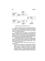
§4.2 The general solution 143
Figure 4.1 The transient cooling of a body as it might occur,
subject to boundary conditions of the first, second, and third
kinds.
This list of b.c.’s is not complete, by any means, but it includes a great
number of important cases.
Figure 4.1 shows the transient cooling of body from a constant initial
temperature, subject to each of the three b.c.’s described above. Notice
that the initial temperature distribution is not subject to the boundary
condition, as pointed out previously under 2(a).
The eight-point procedure that was outlined in Section 2.2 for solving
the heat diffusion equation was contrived in part to assure that a problem
will meet the preceding requirements and will be well posed.
4.2 The general solution
Once the heat conduction problem has been posed properly, the first step
in solving it is to find the general solution of the heat diffusion equation.
We have remarked that this is usually the easiest part of the problem.
We next consider some examples of general solutions.
144 Analysis of heat conduction and some steady one-dimensional problems §4.2
One-dimensional steady heat conduction
Problem 4.1 emphasizes the simplicity of finding the general solutions of
linear ordinary differential equations, by asking for a table of all general
solutions of one-dimensional heat conduction problems. We shall work
out some of those results to show what is involved. We begin the heat
diffusion equation with constant k and
˙
q:
∇
2
T +

˙
q
k
=
1
α
∂T
∂t
(2.11)
Cartesian coordinates: Steady conduction in the y-direction. Equation
(2.11) reduces as follows:
∂
2
T
∂x
2

=0
+
∂
2
T
∂y
2
+
∂
2
T
∂z
2


=0
+
˙
q
k
=
1
α
∂T
∂t

 
= 0, since steady
Therefore,
d
2
T
dy
2
=−
˙
q
k
which we integrate twice to get
T =−
˙
q
2k
y

2
+C
1
y + C
2
or, if
˙
q = 0,
T = C
1
y + C
2
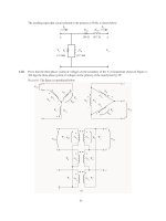
Cylindrical coordinates with a heat source: Tangential conduction.
This time, we look at the heat flow that results in a ring when two points
are held at different temperatures. We now express eqn. (2.11) in cylin-
drical coordinates with the help of eqn. (2.13):
1
r
∂
∂r

r
∂T
∂r


 
=0
+
1

r
2
∂
2
T
∂φ
2
  
r =constant
+
∂
2
T
∂z
2

=0
+
˙
q
k
=
1
α
∂T
∂t

 
= 0, since steady
Two integrations give

T =−
r
2
˙
q
2k
φ
2
+C
1
φ + C
2
(4.1)
This would describe, for example, the temperature distribution in the
thin ring shown in Fig. 4.2. Here the b.c.’s might consist of temperatures
specified at two angular locations, as shown.
§4.2 The general solution 145
Figure 4.2 One-dimensional heat conduction in a ring.
T = T(t only)
If T is spatially uniform, it can still vary with time. In such cases
∇
2
T


=0
+
˙
q
k

=
1
α
∂T
∂t
and ∂T/∂t becomes an ordinary derivative. Then, since α = k/ρc,
dT
dt
=
˙
q
ρc
(4.2)
This result is consistent with the lumped-capacity solution described in
Section 1.3. If the Biot number is low and internal resistance is unimpor-
tant, the convective removal of heat from the boundary of a body can be
prorated over the volume of the body and interpreted as
˙
q
effective
=−
h(T
body
−T
∞
)A
volume
W/m
3
(4.3)

and the heat diffusion equation for this case, eqn. (4.2), becomes
dT
dt
=−
hA
ρcV
(T −T
∞
) (4.4)
The general solution in this situation was given in eqn. (1.21). [A partic-
ular solution was also written in eqn. (1.22).]
146 Analysis of heat conduction and some steady one-dimensional problems §4.2
Separation of variables: A general solution of multidimensional
problems
Suppose that the physical situation permits us to throw out all but one of
the spatial derivatives in a heat diffusion equation. Suppose, for example,
that we wish to predict the transient cooling in a slab as a function of
the location within it. If there is no heat generation, the heat diffusion
equation is
∂
2
T
∂x
2
=
1
α
∂T
∂t
(4.5)

A common trick is to ask: “Can we find a solution in the form of a product
of functions of t and x: T =T(t) ·X(x)?” To find the answer, we
substitute this in eqn. (4.5) and get
X

T=
1
α
T

X (4.6)
where each prime denotes one differentiation of a function with respect
to its argument. Thus T

= dT/dt and X

= d
2
X/dx
2
. Rearranging
eqn. (4.6), we get
X

X
=
1
α
T


T
(4.7a)
This is an interesting result in that the left-hand side depends only
upon x and the right-hand side depends only upon t. Thus, we set both
sides equal to the same constant, which we call −λ
2
, instead of, say, λ,
for reasons that will be clear in a moment:
X

X
=
1
α
T

T
=−λ
2
a constant (4.7b)
It follows that the differential eqn. (4.7a) can be resolved into two ordi-
nary differential equations:
X

=−λ
2
X and T

=−αλ
2

T (4.8)
The general solution of both of these equations are well known and
are among the first ones dealt with in any study of differential equations.
They are:
X(x) = A sinλx + B cos λx for λ ≠ 0
X(x) = Ax + B for λ = 0
(4.9)
§4.2 The general solution 147
and
T (t) = Ce
−αλ
2
t
for λ ≠ 0
T (t) = C for λ = 0
(4.10)
where we use capital letters to denote constants of integration. [In ei-
ther case, these solutions can be verified by substituting them back into
eqn. (4.8).] Thus the general solution of eqn. (4.5) can indeed be written
in the form of a product, and that product is
T =XT =e
−αλ
2
t
(D sin λx +E cos λx) for λ ≠ 0
T =XT =Dx +E for λ = 0
(4.11)
The usefulness of this result depends on whether or not it can be fit
to the b.c.’s and the i.c. In this case, we made the function X(t) take the
form of sines and cosines (instead of exponential functions) by placing

a minus sign in front of λ
2
. The sines and cosines make it possible to fit
the b.c.’s using Fourier series methods. These general methods are not
developed in this book; however, a complete Fourier series solution is
presented for one problem in Section 5.3.
The preceding simple methods for obtaining general solutions of lin-
ear partial d.e.’s is called the method of separation of variables. It can be
applied to all kinds of linear d.e.’s. Consider, for example, two-dimen-
sional steady heat conduction without heat sources:
∂
2
T
∂x
2
+
∂
2
T
∂y
2
= 0 (4.12)
Set T =XYand get
X

X
=−
Y

Y

=−λ
2
where λ can be an imaginary number. Then
X=A sin λx + B cos λx
Y=Ce
λy
+De
−λy



for λ ≠ 0
X=Ax +B
Y=Cy + D

for λ = 0
The general solution is
T = (E sinλx + F cos λx)(e
−λy
+Ge
λy
) for λ ≠ 0
T = (Ex +F)(y +G) for λ = 0
(4.13)
148 Analysis of heat conduction and some steady one-dimensional problems §4.2
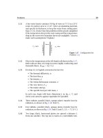
Figure 4.3 A two-dimensional slab maintained at a constant
temperature on the sides and subjected to a sinusoidal varia-
tion of temperature on one face.
Example 4.1
A long slab is cooled to 0

◦
C on both sides and a blowtorch is turned
on the top edge, giving an approximately sinusoidal temperature dis-
tribution along the top, as shown in Fig. 4.3. Find the temperature
distribution within the slab.
Solution. The general solution is given by eqn. (4.13). We must
therefore identify the appropriate b.c.’s and then fit the general solu-
tion to it. Those b.c.’s are:
on the top surface : T(x,0) = A sin π
x
L
on the sides : T(0orL, y) = 0
as y →∞: T(x,y →∞) = 0
Substitute eqn. (4.13) in the third b.c.:
(E sin λx +F cos λx)(0 +G ·∞) = 0
The only way that this can be true for all x is if G = 0. Substitute
eqn. (4.13), with G = 0, into the second b.c.:
(O + F)e
−λy
= 0
§4.2 The general solution 149
so F also equals 0. Substitute eqn. (4.13) with G = F = 0, into the first
b.c.:
E(sin λx) = A sinπ
x
L
It follows that A = E and λ = π/L. Then eqn. (4.13) becomes the
particular solution that satisfies the b.c.’s:
T = A


sin π
x
L

e
−πy/L
Thus, the sinusoidal variation of temperature at the top of the slab is
attenuated exponentially at lower positions in the slab. At a position
of y = 2L below the top, T will be 0.0019 A sin πx/L. The tempera-
ture distribution in the x-direction will still be sinusoidal, but it will
have less than 1/500 of the amplitude at y = 0.
Consider some important features of this and other solutions:
• The b.c. at y = 0 is a special one that works very well with this
particular general solution. If we had tried to fit the equation to
a general temperature distribution, T(x,y = 0) = fn(x), it would
not have been obvious how to proceed. Actually, this is the kind
of problem that Fourier solved with the help of his Fourier series
method. We discuss this matter in more detail in Chapter 5.
• Not all forms of general solutions lend themselves to a particular
set of boundary and/or initial conditions. In this example, we made
the process look simple, but more often than not, it is in fitting a
general solution to a set of boundary conditions that we get stuck.
• Normally, on formulating a problem, we must approximate real be-
havior in stating the b.c.’s. It is advisable to consider what kind of
assumption will put the b.c.’s in a form compatible with the gen-
eral solution. The temperature distribution imposed on the slab
by the blowtorch in Example 4.1 might just as well have been ap-
proximated as a parabola. But as small as the difference between a
parabola and a sine function might be, the latter b.c. was far easier
to accommodate.

• The twin issues of existence and uniqueness of solutions require
a comment here: It has been established that solutions to all well-
posed heat diffusion problems are unique. Furthermore, we know
150 Analysis of heat conduction and some steady one-dimensional problems §4.3
from our experience that if we describe a physical process correctly,
a unique outcome exists. Therefore, we are normally safe to leave
these issues to a mathematician—at least in the sort of problems
we discuss here.
• Given that a unique solution exists, we accept any solution as cor-
rect since we have carved it to fit the boundary conditions. In this
sense, the solution of differential equations is often more of an in-
centive than a formal operation. The person who does it best is
often the person who has done it before and so has a large assort-
ment of tricks up his or her sleeve.
4.3 Dimensional analysis
Introduction
Most universities place the first course in heat transfer after an introduc-
tion to fluid mechanics: and most fluid mechanics courses include some
dimensional analysis. This is normally treated using the familiar method
of indices, which is seemingly straightforward to teach but is cumber-
some and sometimes misleading to use. It is rather well presented in
[4.1].
The method we develop here is far simpler to use than the method
of indices, and it does much to protect us from the common errors we
might fall into. We refer to it as the method of functional replacement.
The importance of dimensional analysis to heat transfer can be made
clearer by recalling Example 2.6, which (like most problems in Part I) in-
volved several variables. Theses variables included the dependent vari-
able of temperature, (T
∞

− T
i
);
3
the major independent variable, which
was the radius, r; and five system parameters, r
i
,r
o
, h,k, and (T
∞
−T
i
).
By reorganizing the solution into dimensionless groups [eqn. (2.24)], we
reduced the total number of variables to only four:
T −T
i
T
∞
−T
i
  
dependent variable
= fn



r


r
i
,

 
indep. var.
r
o

r
i
, Bi

 
two system parameters



(2.24a)
3
Notice that we do not call T
i
a variable. It is simply the reference temperature
against which the problem is worked. If it happened to be 0
◦
C, we would not notice its
subtraction from the other temperatures.
§4.3 Dimensional analysis 151
This solution offered a number of advantages over the dimensional
solution. For one thing, it permitted us to plot all conceivable solutions

for a particular shape of cylinder, (r
o
/r
i
), in a single figure, Fig. 2.13.
For another, it allowed us to study the simultaneous roles of
h, k and r
o
in defining the character of the solution. By combining them as a Biot
number, we were able to say—even before we had solved the problem—
whether or not external convection really had to be considered.
The nondimensionalization made it possible for us to consider, simul-
taneously, the behavior of all similar systems of heat conduction through
cylinders. Thus a large, highly conducting cylinder might be similar in
its behavior to a small cylinder with a lower thermal conductivity.
Finally, we shall discover that, by nondimensionalizing a problem be-
fore we solve it, we can often greatly simplify the process of solving it.
Our next aim is to map out a method for nondimensionalization prob-
lems before we have solved then, or, indeed, before we have even written
the equations that must be solved. The key to the method is a result
called the Buckingham pi-theorem.
The Buckingham pi-theorem
The attention of scientific workers was apparently drawn very strongly
toward the question of similarity at about the beginning of World War I.
Buckingham first organized previous thinking and developed his famous
theorem in 1914 in the Physical Review [4.2], and he expanded upon the
idea in the Transactions of the ASME one year later [4.3]. Lord Rayleigh
almost simultaneously discussed the problem with great clarity in 1915
[4.4]. To understand Buckingham’s theorem, we must first overcome one
conceptual hurdle, which, if it is clear to the student, will make everything

that follows extremely simple. Let us explain that hurdle first.
Suppose that y depends on r,x,z and so on:
y = y(r,x,z, )
We can take any one variable—say, x—and arbitrarily multiply it (or it
raised to a power) by any other variables in the equation, without altering
the truth of the functional equation, like this:
y
x
=
y
x

x
2
r,x,xz

To see that this is true, consider an arbitrary equation:
y = y(r,x,z) = r(sin x)e
−z
152 Analysis of heat conduction and some steady one-dimensional problems §4.3
This need only be rearranged to put it in terms of the desired modified
variables and x itself (y/x, x
2
r,x, and xz):
y
x
=
x
2
r

x
3
(sin x)exp

−
xz
x

We can do any such multiplying or dividing of powers of any variable
we wish without invalidating any functional equation that we choose to
write. This simple fact is at the heart of the important example that
follows:
Example 4.2
Consider the heat exchanger problem described in Fig. 3.15. The “un-
known,” or dependent variable, in the problem is either of the exit
temperatures. Without any knowledge of heat exchanger analysis, we
can write the functional equation on the basis of our physical under-
standing of the problem:
T
c
out
−T
c
in
  
K
= fn





C
max
  
W/K
,C
min
 
W/K
,

T
h
in
−T
c
in


 
K
,U

 
W/m
2
K
,A

m

2




(4.14)
where the dimensions of each term are noted under the quotation.
We want to know how many dimensionless groups the variables in
eqn. (4.14) should reduce to. To determine this number, we use the
idea explained above—that is, that we can arbitrarily pick one vari-
able from the equation and divide or multiply it into other variables.
Then—one at a time—we select a variable that has one of the dimen-
sions. We divide or multiply it by the other variables in the equation
that have that dimension in such a way as to eliminate the dimension
from them.
We do this first with the variable (T
h
in
− T
c
in
), which has the di-
mension of K.
T
c
out
−T
c
in
T

h
in
−T
c
in
  
dimensionless
= fn



C
max
(T
h
in
−T
c
in
)

 
W
,C
min
(T
h
in
−T
c

in
)

 
W
,
(T
h
in
−T
c
in
)

 
K
,U(T
h
in
−T
c
in
)

 
W/m
2
,A

m

2




§4.3 Dimensional analysis 153
The interesting thing about the equation in this form is that the only
remaining term in it with the units of K is (T
h
in
− T
c
in
). No such
term can exist in the equation because it is impossible to achieve
dimensional homogeneity without another term in K to balance it.
Therefore, we must remove it.
T
c
out
−T
c
in
T
h
in
−T
c
in
  

dimensionless
= fn




C
max
(T
h
in
−T
c
in
)

 
W
,C
min
(T
h
in
−T
c
in
)

 
W

,U(T
h
in
−T
c
in
)

 
W/m
2
,A

m
2




Now the equation has only two dimensions in it—W and m
2
. Next, we
multiply U(T
h
in
−T
c
in
) by A to get rid of m
2

in the second-to-last term.
Accordingly, the term A (m
2
) can no longer stay in the equation, and
we have
T
c
out
−T
c
in
T
h
in
−T
c
in
  
dimensionless
= fn



C
max
(T
h
in
−T
c

in
)

 
W
,C
min
(T
h
in
−T
c
in
)

 
W
, UA(T
h
in
−T
c
in
)

 
W
,




Next, we divide the first and third terms on the right by the second.
This leaves only C
min
(T
h
in
−T
c
in
), with the dimensions of W. That term
must then be removed, and we are left with the completely dimension-
less result:
T
c
out
−T
c
in
T
h
in
−T
c
in
= fn

C
max
C

min
,
UA
C
min

(4.15)
Equation (4.15) has exactly the same functional form as eqn. (3.21),
which we obtained by direct analysis.
Notice that we removed one variable from eqn. (4.14) for each di-
mension in which the variables are expressed. If there are n variables—
including the dependent variable—expressed in m dimensions, we then
expect to be able to express the equation in (n − m) dimensionless
groups, or pi-groups, as Buckingham called them.
This fact is expressed by the Buckingham pi-theorem, which we state
formally in the following way:
154 Analysis of heat conduction and some steady one-dimensional problems §4.3
A physical relationship among n variables, which can be ex-
pressed in a minimum of m dimensions, can be rearranged into
a relationship among (n −m) independent dimensionless groups
of the original variables.
Two important qualifications have been italicized. They will be explained
in detail in subsequent examples.
Buckingham called the dimensionless groups pi-groups and identified
them as Π
1
, Π
2
, ,Π
n−m

. Normally we call Π
1
the dependent variable
and retain Π
2→(n−m)
as independent variables. Thus, the dimensional
functional equation reduces to a dimensionless functional equation of
the form
Π
1
= fn
(
Π
2
, Π
3
, ,Π
n−m
)
(4.16)
Applications of the pi-theorem
Example 4.3
Is eqn. (2.24) consistent with the pi-theorem?
Solution. To find out, we first write the dimensional functional
equation for Example 2.6:
T −T
i
  
K
= fn


r

m
,r
i

m
,r
o

m
, h

 
W/m
2
K
,k

 
W/m·K
,(T
∞
−T
i
)

 
K


There are seven variables (n = 7) in three dimensions, K, m, and W
(m = 3). Therefore, we look for 7 −3 = 4 pi-groups. There are four
pi-groups in eqn. (2.24):
Π
1
=
T −T
i
T
∞
−T
i
, Π
2
=
r
r
i
, Π
3
=
r
o
r
i
, Π
4
=
hr

o
k
≡ Bi.
Consider two features of this result. First, the minimum number of
dimensions was three. If we had written watts as J/s, we would have
had four dimensions instead. But Joules never appear in that particular
problem independently of seconds. They always appear as a ratio and
should not be separated. (If we had worked in English units, this would
have seemed more confusing, since there is no name for Btu/sec unless
§4.3 Dimensional analysis 155
we first convert it to horsepower.) The failure to identify dimensions
that are consistently grouped together is one of the major errors that the
beginner makes in using the pi-theorem.
The second feature is the independence of the groups. This means
that we may pick any four dimensionless arrangements of variables, so
long as no group or groups can be made into any other group by math-
ematical manipulation. For example, suppose that someone suggested
that there was a fifth pi-group in Example 4.3:
Π
5
=

hr
k
It is easy to see that Π
5
can be written as
Π
5
=


hr
o
k

r
r
i

r
i
r
o
=

Bi
Π
2
Π
3
Therefore Π
5
is not independent of the existing groups, nor will we ever
find a fifth grouping that is.
Another matter that is frequently made much of is that of identifying
the pi-groups once the variables are identified for a given problem. (The
method of indices [4.1] is a cumbersome arithmetic strategy for doing
this but it is perfectly correct.) We shall find the groups by using either
of two methods:
1. The groups can always be obtained formally by repeating the simple

elimination-of-dimensions procedure that was used to derive the
pi-theorem in Example 4.2.
2. One may simply arrange the variables into the required number of
independent dimensionless groups by inspection.
In any method, one must make judgments in the process of combining
variables and these decisions can lead to different arrangements of the
pi-groups. Therefore, if the problem can be solved by inspection, there
is no advantage to be gained by the use of a more formal procedure.
The methods of dimensional analysis can be used to help find the
solution of many physical problems. We offer the following example,
not entirely with tongue in cheek:
Example 4.4
Einstein might well have noted that the energy equivalent, e, of a rest
156 Analysis of heat conduction and some steady one-dimensional problems §4.3
mass, m
o
, depended on the velocity of light, c
o
, before he developed
the special relativity theory. He wold then have had the following
dimensional functional equation:

e N·more
kg· m
2
s
2

= fn
(

c
o
m/s,m
o
kg
)
The minimum number of dimensions is only two: kg and m/s, so we
look for 3 − 2 = 1 pi-group. To find it formally, we eliminated the
dimension of mass from e by dividing it by m
o
(kg). Thus,
e
m
o
m
2
s
2
= fn

c
o
m/s,m
o
kg

 
this must be removed
because it is the only
term with mass in it


Then we eliminate the dimension of velocity (m/s) by dividing e/m
o
by c
2
o
:
e
m
o
c
2
o
= fn
(
c
o
m/s
)
This time c
o
must be removed from the function on the right, since it
is the only term with the dimensions m/s. This gives the result (which
could have been written by inspection once it was known that there
could only be one pi-group):
Π
1
=
e
m

o
c
2
o
= fn
(
no other groups
)
= constant
or
e = constant ·

m
o
c
2
o

Of course, it required Einstein’s relativity theory to tell us that the
constant is unity.
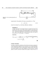
Example 4.5
What is the velocity of efflux of liquid from the tank shown in Fig. 4.4?
Solution. In this case we can guess that the velocity, V, might de-
pend on gravity, g, and the head H. We might be tempted to include
§4.3 Dimensional analysis 157
Figure 4.4 Efflux of liquid
from a tank.
the density as well until we realize that g is already a force per unit
mass. To understand this, we can use English units and divide g by the
conversion factor,

4
g
c
. Thus (g ft/s
2
)/(g
c
lb
m
·ft/lb
f
s
2
)=g lb
f
/lb
m
.
Then
V

m/s
= fn

H

m
,g

m/s

2

so there are three variables in two dimensions, and we look for 3−2 =
1 pi-groups. It would have to be
Π
1
=
V

gH
= fn
(
no other pi-groups
)
= constant
or
V = constant ·

gH
The analytical study of fluid mechanics tells us that this form is
correct and that the constant is
√
2. The group V
2
/gh, by the way, is
called a Froude number, Fr (pronounced “Frood”). It compares inertial
forces to gravitational forces. Fr is about 1000 for a pitched baseball,
and it is between 1 and 10 for the water flowing over the spillway of
a dam.
4

One can always divide any variable by a conversion factor without changing it.
158 Analysis of heat conduction and some steady one-dimensional problems §4.3
Example 4.6
Obtain the dimensionless functional equation for the temperature
distribution during steady conduction in a slab with a heat source,
˙
q.
Solution. In such a case, there might be one or two specified tem-
peratures in the problem: T
1
or T
2
. Thus the dimensional functional
equation is
T −T
1
  
K
= fn




(T
2
−T
1
)

 

K
,x,L


m
,
˙
q

W/m
3
,k

 
W/m·K
, h

 
W/m
2
K




where we presume that a convective b.c. is involved and we identify a
characteristic length, L, in the x-direction. There are seven variables
in three dimensions, or 7 − 3 = 4 pi-groups. Three of these groups
are ones we have dealt with in the past in one form or another:
Π

1
=
T −T
1
T
2
−T
1
dimensionless temperature, which we
shall give the name Θ
Π
2
=
x
L
dimensionless length, which we call ξ
Π
3
=
hL
k
which we recognize as the Biot number, Bi
The fourth group is new to us:
Π
4
=
˙
qL
2
k(T

2
−T
1
)
which compares the heat generation rate to
the rate of heat loss; we call it Γ
Thus, the solution is
Θ = fn
(
ξ,Bi, Γ
)
(4.17)
In Example 2.1, we undertook such a problem, but it differed in two
respects. There was no convective boundary condition and hence, no
h,
and only one temperature was specified in the problem. In this case, the
dimensional functional equation was
(
T −T
1
)
= fn

x,L,
˙
q, k

so there were only five variables in the same three dimensions. The re-
sulting dimensionless functional equation therefore involved only two
§4.4 An illustration of dimensional analysis in a complex steady conduction problem 159

pi-groups. One was ξ = x/L and the other is a new one equal to Θ/Γ .We
call it Φ:
Φ ≡
T −T
1
˙
qL
2
/k
= fn

x
L

(4.18)
And this is exactly the form of the analytical result, eqn. (2.15).
Finally, we must deal with dimensions that convert into one another.
For example, kg and N are defined in terms of one another through New-
ton’s Second Law of Motion. Therefore, they cannot be identified as sep-
arate dimensions. The same would appear to be true of J and N·m, since
both are dimensions of energy. However, we must discern whether or
not a mechanism exists for interchanging them. If mechanical energy
remains distinct from thermal energy in a given problem, then J should
not be interpreted as N·m.
This issue will prove important when we do the dimensional anal-
ysis of several heat transfer problems. See, for example, the analyses
of laminar convection problem at the beginning of Section 6.4, of natu-
ral convection in Section 8.3, of film condensation in Section 8.5, and of
pool boiling burnout in Section 9.3. In all of these cases, heat transfer
normally occurs without any conversion of heat to work or work to heat

and it would be misleading to break J into N·m.
Additional examples of dimensional analysis appear throughout this
book. Dimensional analysis is, indeed, our court of first resort in solving
most of the new problems that we undertake.
4.4 An illustration of the use of dimensional analysis
in a complex steady conduction problem
Heat conduction problems with convective boundary conditions can rap-
idly grow difficult, even if they start out simple, and so we look for ways
to avoid making mistakes. For one thing, it is wise to take great care
that dimensions are consistent at each stage of the solution. The best
way to do this, and to eliminate a great deal of algebra at the same time,
is to nondimensionalize the heat conduction equation before we apply
the b.c.’s. This nondimensionalization should be consistent with the pi-
theorem. We illustrate this idea with a fairly complex example.
160 Analysis of heat conduction and some steady one-dimensional problems §4.4
Figure 4.5 Heat conduction through a heat-generating slab
with asymmetric boundary conditions.
Example 4.7
A slab shown in Fig. 4.5 has different temperatures and different heat
transfer coefficients on either side and the heat is generated within
it. Calculate the temperature distribution in the slab.
Solution. The differential equation is
d
2
T
dx
2
=−
˙
q

k
and the general solution is
T =−
˙
qx
2
2k
+C
1
x + C
2
(4.19)
§4.4 An illustration of dimensional analysis in a complex steady conduction problem 161
with b.c.’s
h
1
(T
1
−T)
x=0
=−k
dT
dx




x=0
, h
2

(T −T
2
)
x=L
=−k
dT
dx




x=L
.
(4.20)
There are eight variables involved in the problem: (T −T
2
), (T
1
−T
2
),
x, L, k,
h
1
, h
2
, and
˙
q; and there are three dimensions: K, W, and m.
This results in 8 − 3 = 5 pi-groups. For these we choose

Π
1
≡ Θ =
T −T
2
T
1
−T
2
, Π
2
≡ ξ =
x
L
, Π
3
≡ Bi
1
=
h
1
L
k
,
Π
4
≡ Bi
2
=
h

2
L
k
, and Π
5
≡ Γ =
˙
qL
2
2k(T
1
−T
2
)
,
where Γ can be interpreted as a comparison of the heat generated in
the slab to that which could flow through it.
Under this nondimensionalization, eqn. (4.19) becomes
5
Θ =−Γ ξ
2
+C
3
ξ + C
4
(4.21)
and b.c.’s become
Bi
1
(1 − Θ

ξ=0
) =−Θ

ξ=0
, Bi
2
Θ
ξ=1
=−Θ

ξ=1
(4.22)
where the primes denote differentiation with respect to ξ. Substitut-
ing eqn. (4.21) in eqn. (4.22), we obtain
Bi
1
(1 − C
4
) =−C
3
, Bi
2
(−Γ +C
3
+C
4
) = 2Γ −C
3
. (4.23)
Substituting the first of eqns. (4.23) in the second we get

C
4
= 1 +
−Bi
1
+2(Bi
1
/Bi
2
)Γ +Bi
1
Γ
Bi
1
+Bi
2
1

Bi
2
+Bi
2
1
C
3
= Bi
1
(C
4
−1)

Thus, eqn. (4.21) becomes
Θ = 1 + Γ

2(Bi
1

Bi
2
) + Bi
1
1 + Bi
1

Bi
2
+Bi
1
ξ − ξ
2
+
2(Bi
1

Bi
2
) + Bi
1
Bi
1
+Bi

2
1

Bi
2
+Bi
2
1

−
Bi
1
1 + Bi
1

Bi
2
+Bi
1
ξ −
Bi
1
Bi
1
+Bi
2
1

Bi
2

+Bi
2
1
(4.24)
5
The rearrangement of the dimensional equations into dimensionless form is
straightforward algebra. If the results shown here are not immediately obvious to
you, sketch the calculation on a piece of paper.
162 Analysis of heat conduction and some steady one-dimensional problems §4.4
This is a complicated result and one that would have required enormous
patience and accuracy to obtain without first simplifying the problem
statement as we did. If the heat transfer coefficients were the same on
either side of the wall, then Bi
1
= Bi
2
≡ Bi, and eqn. (4.24) would reduce
to
Θ = 1 + Γ

ξ − ξ
2
+1/Bi

−
ξ + 1/Bi
1 + 2/Bi
(4.25)
which is a very great simplification.
Equation (4.25) is plotted on the left-hand side of Fig. 4.5 for Bi equal

to 0, 1, and ∞ and for Γ equal to 0, 0.1, and 1. The following features
should be noted:
• When Γ  0.1, the heat generation can be ignored.
• When Γ  1, Θ → Γ /Bi + Γ (ξ − ξ
2
). This is a simple parabolic tem-
perature distribution displaced upward an amount that depends on
the relative external resistance, as reflected in the Biot number.
• If both Γ and 1/Bi become large, Θ → Γ /Bi. This means that when
internal resistance is low and the heat generation is great, the slab
temperature is constant and quite high.
If T
2
were equal to T
1
in this problem, Γ would go to infinity. In such
a situation, we should redo the dimensional analysis of the problem. The
dimensional functional equation now shows (T −T
1
) to be a function of
x, L, k,
h, and
˙
q. There are six variables in three dimensions, so there
are three pi-groups
T −T
1
˙
qL/h
= fn

(
ξ,Bi
)
where the dependent variable is like Φ [recall eqn. (4.18)] multiplied by
Bi. We can put eqn. (4.25) in this form by multiplying both sides of it by
h(T
1
−T
2
)/
˙
qδ. The result is
h(T −T
1
)
˙
qL
=
1
2
Bi

ξ − ξ
2

+
1
2
(4.26)
The result is plotted on the right-hand side of Fig. 4.5. The following

features of the graph are of interest:
• Heat generation is the only “force” giving rise to temperature nonuni-
formity. Since it is symmetric, the graph is also symmetric.
§4.5 Fin design 163
• When Bi  1, the slab temperature approaches a uniform value
equal to T
1
+
˙
qL/2h. (In this case, we would have solved the prob-
lem with far greater ease by using a simple lumped-capacity heat
balance, since it is no longer a heat conduction problem.)
• When Bi > 100, the temperature distribution is a very large parabola
with ½ added to it. In this case, the problem could have been solved
using boundary conditions of the first kind because the surface
temperature stays very close to T
∞
(recall Fig. 1.11).
4.5 Fin design
The purpose of fins
The convective removal of heat from a surface can be substantially im-
proved if we put extensions on that surface to increase its area. These
extensions can take a variety of forms. Figure 4.6, for example, shows
many different ways in which the surface of commercial heat exchanger
tubing can be extended with protrusions of a kind we call fins.
Figure 4.7 shows another very interesting application of fins in a heat
exchanger design. This picture is taken from an issue of Science maga-
zine [4.5], which presents an intriguing argument by Farlow, Thompson,
and Rosner. They offered evidence suggesting that the strange rows of
fins on the back of the Stegosaurus were used to shed excess body heat

after strenuous activity, which is consistent with recent suspicions that
Stegosaurus was warm-blooded.
These examples involve some rather complicated fins. But the analy-
sis of a straight fin protruding from a wall displays the essential features
of all fin behavior. This analysis has direct application to a host of prob-
lems.
Analysis of a one-dimensional fin
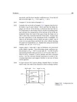
The equations. Figure 4.8 shows a one-dimensional fin protruding from
a wall. The wall—and the roots of the fin—are at a temperature T
0
, which
is either greater or less than the ambient temperature, T
∞
. The length
of the fin is cooled or heated through a heat transfer coefficient,
h,by
the ambient fluid. The heat transfer coefficient will be assumed uniform,
although (as we see in Part III) that can introduce serious error in boil-