A HEAT TRANSFER TEXTBOOK - THIRD EDITION Episode 1 Part 10 pdf

214 Transient and multidimensional heat conduction §5.4
Solution. After 1 hr, or 3600 s:
Fo =
αt
r
2
o
=

k
ρc

20
◦
C
3600 s
(0.05 m)
2
=
(0.603 J/m·s·K)(3600 s)
(997.6 kg/m
3
)(4180 J/kg·K)(0.0025 m
2
)
= 0.208
Furthermore, Bi
−1
= (hr
o
/k)

−1
= [6(0.05)/0.603]
−1
= 2.01. There-
fore, we read from Fig. 5.9 in the upper left-hand corner:
Θ = 0.85
After 1 hr:
T
center
= 0.85(30 −5)
◦
C +5
◦
C = 26.3
◦
C
To find the time required to bring the center to 10
◦
C, we first
calculate
Θ =
10 −5
30 −5
= 0.2
and Bi
−1
is still 2.01. Then from Fig. 5.9 we read
Fo = 1.29 =
αt
r

2
o
so
t =
1.29(997.6)(4180)(0.0025)
0.603
= 22, 300 s = 6hr12min
Finally, we look up Φ at Bi = 1/2.01 and Fo = 1.29 in Fig. 5.10, for
spheres:
Φ = 0.80 =

t
0
Qdt
ρc

4
3
πr
3
0

(T
i
−T
∞
)
so

t

0
Qdt = 997.6(4180)

4
3
π(0.05)
3

(25)(0.80) = 43, 668 J/apple
Therefore, for the 12 apples,
total energy removal = 12(43.67) = 524 kJ
§5.4 Temperature-response charts 215
The temperature-response charts in Fig. 5.7 through Fig. 5.10 are with-
out doubt among the most useful available since they can be adapted to
a host of physical situations. Nevertheless, hundreds of such charts have
been formed for other situations, a number of which have been cataloged
by Schneider [5.5]. Analytical solutions are available for hundreds more
problems, and any reader who is faced with a complex heat conduction
calculation should consult the literature before trying to solve it. An ex-
cellent place to begin is Carslaw and Jaeger’s comprehensive treatise on
heat conduction [5.6].
Example 5.3
A 1 mm diameter Nichrome (20% Ni, 80% Cr) wire is simultaneously
being used as an electric resistance heater and as a resistance ther-
mometer in a liquid flow. The laboratory workers who operate it are
attempting to measure the boiling heat transfer coefficient,
h, by sup-
plying an alternating current and measuring the difference between
the average temperature of the heater, T
av

, and the liquid tempera-
ture, T
∞
. They get h = 30, 000 W/m
2
K at a wire temperature of 100
◦
C
and are delighted with such a high value. Then a colleague suggests
that
h is so high because the surface temperature is rapidly oscillating
as a result of the alternating current. Is this hypothesis correct?
Solution. Heat is being generated in proportion to the product of
voltage and current, or as sin
2
ωt, where ω is the frequency of the
current in rad/s. If the boiling action removes heat rapidly enough in
comparison with the heat capacity of the wire, the surface tempera-
ture may well vary significantly. This transient conduction problem
was first solved by Jeglic in 1962 [5.7]. It was redone in a different
form two years later by Switzer and Lienhard (see, e.g. [5.8]), who gave
response curves in the form
T
max
−T
av
T
av
−T
∞

= fn
(
Bi,ψ
)
(5.41)
where the left-hand side is the dimensionless range of the tempera-
ture oscillation, and ψ = ωδ
2
/α, where δ is a characteristic length
[see Problem 5.56]. Because this problem is common and the solu-
tion is not widely available, we include the curves for flat plates and
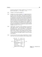
cylinders in Fig. 5.11 and Fig. 5.12 respectively.
Figure 5.11 Temperature deviation at the surface of a flat plate heated with alternating current.
216
Figure 5.12 Temperature deviation at the surface of a cylinder heated with alternating current.
217
218 Transient and multidimensional heat conduction §5.5
In the present case:
Bi =
h radius
k
=
30, 000(0.0005)
13.8
= 1.09
ωr
2
α
=
[2π(60)](0.0005)

2
0.00000343
= 27.5
and from the chart for cylinders, Fig. 5.12, we find that
T
max
−T
av
T
av
−T
∞
 0.04
A temperature fluctuation of only 4% is probably not serious. It there-
fore appears that the experiment was valid.
5.5 One-term solutions
As we have noted previously, when the Fourier number is greater than 0.2
or so, the series solutions from eqn. (5.36) may be approximated using
only their first term:
Θ ≈ A
1
·f
1
·exp

−
ˆ
λ
2
1

Fo

. (5.42)
Likewise, the fractional heat loss, Φ, or the mean temperature
Θ from
eqn. (5.40), can be approximated using just the first term of eqn. (5.38):
Θ = 1 − Φ ≈ D
1
exp

−
ˆ
λ
2
1
Fo

. (5.43)
Table 5.2 lists the values of
ˆ
λ
1
, A
1
, and D
1
for slabs, cylinders, and
spheres as a function of the Biot number. The one-term solution’s er-
ror in Θ is less than 0.1% for a sphere with Fo ≥ 0.28 and for a slab with
Fo ≥ 0.43. These errors are largest for Biot numbers near unity. If high

accuracy is not required, these one-term approximations may generally
be used whenever Fo ≥ 0.2
Table 5.2 One-term coefficients for convective cooling [5.1].
Plate Cylinder Sphere
Bi
ˆ
λ
1
A
1
D
1
ˆ
λ
1
A
1
D
1
ˆ
λ
1
A
1
D
1
0.01 0.09983 1.0017 1.0000 0.14124 1.0025 1.0000 0.17303 1.0030 1.0000
0.02 0.14095 1.0033 1.0000 0.19950 1.0050 1.0000 0.24446 1.0060 1.0000
0.05 0.22176 1.0082 0.9999 0.31426 1.0124 0.9999 0.38537 1.0150 1.0000
0.10 0.31105 1.0161 0.9998 0.44168 1.0246 0.9998 0.54228 1.0298 0.9998

0.15 0.37788 1.0237 0.9995 0.53761 1.0365 0.9995 0.66086 1.0445 0.9996
0.20 0.43284 1.0311 0.9992 0.61697 1.0483 0.9992 0.75931 1.0592 0.9993
0.30 0.52179 1.0450 0.9983 0.74646 1.0712 0.9983 0.92079 1.0880 0.9985
0.40 0.59324 1.0580 0.9971 0.85158 1.0931 0.9970 1.05279 1.1164 0.9974
0.50 0.65327 1.0701 0.9956 0.94077 1.1143 0.9954 1.16556 1.1441 0.9960
0.60 0.70507 1.0814 0.9940 1.01844 1.1345 0.9936 1.26440 1.1713 0.9944
0.70 0.75056 1.0918 0.9922 1.08725 1.1539 0.9916 1.35252 1.1978 0.9925
0.80 0.79103 1.1016 0.9903 1.14897 1.1724 0.9893 1.43203 1.2236 0.9904
0.90 0.82740 1.1107 0.9882 1.20484 1.1902 0.9869 1.50442 1.2488 0.9880
1.00 0.86033 1.1191 0.9861 1.25578 1.2071 0.9843 1.57080 1.2732 0.9855
1.10 0.89035 1.1270 0.9839 1.30251 1.2232 0.9815 1.63199 1.2970 0.9828
1.20 0.91785 1.1344 0.9817 1.34558 1.2387 0.9787 1.68868 1.3201 0.9800
1.30 0.94316 1.1412 0.9794 1.38543 1.2533 0.9757 1.74140 1.3424 0.9770
1.40 0.96655 1.1477 0.9771 1.42246 1.2673 0.9727 1.79058 1.3640 0.9739
1.50 0.98824 1.1537 0.9748 1.45695 1.2807 0.9696 1.83660 1.3850 0.9707
1.60 1.00842 1.1593 0.9726 1.48917 1.2934 0.9665 1.87976 1.4052 0.9674
1.80 1.04486 1.1695 0.9680 1.54769 1.3170 0.9601 1.95857 1.4436 0.9605
2.00 1.07687 1.1785 0.9635 1.59945 1.3384 0.9537 2.02876 1.4793 0.9534
2.20 1.10524 1.1864 0.9592 1.64557 1.3578 0.9472 2.09166 1.5125 0.9462
2.40 1.13056 1.1934 0.9549 1.68691 1.3754 0.9408 2.14834 1.5433 0.9389
3.00 1.19246 1.2102 0.9431 1.78866 1.4191 0.9224 2.28893 1.6227 0.9171
4.00 1.26459 1.2287 0.9264 1.90808 1.4698 0.8950 2.45564 1.7202 0.8830
5.00 1.31384 1.2402 0.9130 1.98981 1.5029 0.8721 2.57043 1.7870 0.8533
6.00 1.34955 1.2479 0.9021 2.04901 1.5253 0.8532 2.65366 1.8338 0.8281
8.00 1.39782 1.2570 0.8858 2.12864 1.5526 0.8244 2.76536 1.8920 0.7889
10.00 1.42887 1.2620 0.8743 2.17950 1.5677 0.8039 2.83630 1.9249 0.7607
20.00 1.49613 1.2699 0.8464 2.28805 1.5919 0.7542 2.98572 1.9781 0.6922
50.00 1.54001 1.2727 0.8260 2.35724 1.6002 0.7183 3.07884 1.9962 0.6434
100.00 1.55525 1.2731 0.8185 2.38090 1.6015 0.7052 3.11019 1.9990 0.6259
∞ 1.57080 1.2732 0.8106 2.40483 1.6020 0.6917 3.14159 2.0000 0.6079

219
220 Transient and multidimensional heat conduction §5.6
5.6 Transient heat conduction to a semi-infinite
region
Introduction
Bronowksi’s classic television series, The Ascent of Man [5.9], included
a brilliant reenactment of the ancient ceremonial procedure by which
the Japanese forged Samurai swords (see Fig. 5.13). The metal is heated,
folded, beaten, and formed, over and over, to create a blade of remarkable
toughness and flexibility. When the blade is formed to its final configu-
ration, a tapered sheath of clay is baked on the outside of it, so the cross
section is as shown in Fig. 5.13. The red-hot blade with the clay sheath is
then subjected to a rapid quenching, which cools the uninsulated cutting
edge quickly and the back part of the blade very slowly. The result is a
layer of case-hardening that is hardest at the edge and less hard at points
farther from the edge.
Figure 5.13 The ceremonial case-hardening of a Samurai sword.
§5.6 Transient heat conduction to a semi-infinite region 221
Figure 5.14 The initial cooling of a thin
sword blade. Prior to t = t
4
, the blade
might as well be infinitely thick insofar as
cooling is concerned.
The blade is then tough and ductile, so it will not break, but has a fine
hard outer shell that can be honed to sharpness. We need only look a
little way up the side of the clay sheath to find a cross section that was
thick enough to prevent the blade from experiencing the sudden effects
of the cooling quench. The success of the process actually relies on the
failure of the cooling to penetrate the clay very deeply in a short time.

Now we wish to ask: “How can we say whether or not the influence
of a heating or cooling process is restricted to the surface of a body?”
Or if we turn the question around: “Under what conditions can we view
the depth of a body as infinite with respect to the thickness of the region
that has felt the heat transfer process?”
Consider next the cooling process within the blade in the absence of
the clay retardant and when
h is very large. Actually, our considerations
will apply initially to any finite body whose boundary suddenly changes
temperature. The temperature distribution, in this case, is sketched in
Fig. 5.14 for four sequential times. Only the fourth curve—that for which
t = t
4
—is noticeably influenced by the opposite wall. Up to that time,
the wall might as well have infinite depth.
Since any body subjected to a sudden change of temperature is in-
finitely large in comparison with the initial region of temperature change,
we must learn how to treat heat transfer in this period.
Solution aided by dimensional analysis
The calculation of the temperature distribution in a semi-infinite region
poses a difficulty in that we can impose a definite b.c. at only one position—
the exposed boundary. We shall be able to get around that difficulty in a
nice way with the help of dimensional analysis.
222 Transient and multidimensional heat conduction §5.6
When the one boundary of a semi-infinite region, initially at T = T
i
,
is suddenly cooled (or heated) to a new temperature, T
∞
, as in Fig. 5.14,

the dimensional function equation is
T − T
∞
= fn
[
t, x, α, (T
i
−T
∞
)
]
where there is no characteristic length or time. Since there are five vari-
ables in
◦
C, s, and m, we should look for two dimensional groups.
T − T
∞
T
i
−T
∞
  
Θ
= fn

x
√
αt

 

ζ

(5.44)
The very important thing that we learn from this exercise in dimen-
sional analysis is that position and time collapse into one independent
variable. This means that the heat conduction equation and its b.c.s must
transform from a partial differential equation into a simpler ordinary dif-
ferential equation in the single variable, ζ = x

√
αt. Thus, we transform
each side of
∂
2
T
∂x
2
=
1
α
∂T
∂t
as follows, where we call T
i
−T
∞
≡ ∆T :
∂T
∂t
= (T

i
−T
∞
)
∂Θ
∂t
= ∆T
∂Θ
∂ζ
∂ζ
∂t
= ∆T

−
x
2t
√
αt

∂Θ
∂ζ
;
∂T
∂x
= ∆T
∂Θ
∂ζ
∂ζ
∂x
=

∆T
√
αt
∂Θ
∂ζ
;
and
∂
2
T
∂x
2
=
∆T
√
αt
∂
2
Θ
∂ζ
2
∂ζ
∂x
=
∆T
αt
∂
2
Θ
∂ζ

2
.
Substituting the first and last of these derivatives in the heat conduction
equation, we get
d
2
Θ
dζ
2
=−
ζ
2
dΘ
dζ
(5.45)
Notice that we changed from partial to total derivative notation, since
Θ now depends solely on ζ. The i.c. for eqn. (5.45)is
T(t = 0) = T
i
or Θ
(
ζ →∞
)
= 1 (5.46)
§5.6 Transient heat conduction to a semi-infinite region 223
and the one known b.c. is
T(x = 0) = T
∞
or Θ
(

ζ = 0
)
= 0 (5.47)
If we call dΘ/dζ ≡ χ, then eqn. (5.45) becomes the first-order equa-
tion
dχ
dζ
=−
ζ
2
χ
which can be integrated once to get
χ ≡
dΘ
dζ
= C
1
e
−ζ
2
/4
(5.48)
and we integrate this a second time to get
Θ = C
1

ζ
0
e
−ζ

2
/4
dζ + Θ(0)

 
= 0 according
to the b.c.
(5.49)
The b.c. is now satisfied, and we need only substitute eqn. (5.49)inthe
i.c., eqn. (5.46), to solve for C
1
:
1 = C
1

∞
0
e
−ζ
2
/4
dζ
The definite integral is given by integral tables as
√
π,so
C
1
=
1
√

π
Thus the solution to the problem of conduction in a semi-infinite region,
subject to a b.c. of the first kind is
Θ =
1
√
π

ζ
0
e
−ζ
2
/4
dζ =
2
√
π

ζ/2
0
e
−s
2
ds ≡ erf(ζ/2) (5.50)
The second integral in eqn. (5.50), obtained by a change of variables,
is called the error function (erf). Its name arises from its relationship to
certain statistical problems related to the Gaussian distribution, which
describes random errors. In Table 5.3, we list values of the error function
and the complementary error function, erfc(x) ≡ 1 − erf(x). Equation

(5.50) is also plotted in Fig. 5.15.
224 Transient and multidimensional heat conduction §5.6
Table 5.3 Error function and complementary error function.
ζ

2 erf(ζ/2) erfc(ζ/2)ζ

2 erf(ζ/2) erfc(ζ/2)
0.00 0.00000 1.00000 1.10 0.88021 0.11980
0.05 0.05637 0.94363 1.20 0.91031 0.08969
0.10 0.11246 0.88754 1.30 0.93401 0.06599
0.15 0.16800 0.83200 1.40 0.95229 0.04771
0.20 0.22270 0.77730 1.50 0.96611 0.03389
0.30 0.32863 0.67137 1.60 0.97635 0.02365
0.40 0.42839 0.57161 1.70 0.98379 0.01621
0.50 0.52050 0.47950 1.80 0.98909 0.01091
0.60 0.60386 0.39614 1.8214 0.99000 0.01000
0.70 0.67780 0.32220 1.90 0.99279 0.00721
0.80 0.74210 0.25790 2.00 0.99532 0.00468
0.90 0.79691 0.20309 2.50 0.99959 0.00041
1.00 0.84270 0.15730 3.00 0.99998 0.00002
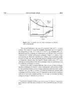
In Fig. 5.15 we see the early-time curves shown in Fig. 5.14 have col-
lapsed into a single curve. This was accomplished by the similarity trans-
formation, as we call it
5
: ζ/2 = x/2
√
αt. From the figure or from Table
5.3, we see that Θ ≥ 0.99 when
ζ

2
=
x
2
√
αt
≥ 1.8214 or x ≥ δ
99
≡ 3.64

αt (5.51)
In other words, the local value of (T −T
∞
) is more than 99% of (T
i
−T
∞
)
for positions in the slab beyond farther from the surface than δ
99
=
3.64
√
αt.
Example 5.4
For what maximum time can a samurai sword be analyzed as a semi-
infinite region after it is quenched, if it has no clay coating and
h
external
∞?

Solution. First, we must guess the half-thickness of the sword (say,
3 mm) and its material (probably wrought iron with an average α
5
The transformation is based upon the “similarity” of spatial an temporal changes
in this problem.
§5.6 Transient heat conduction to a semi-infinite region 225
Figure 5.15 Temperature distribution in
a semi-infinite region.
around 1.5 × 10
−5
m
2
/s). The sword will be semi-infinite until δ
99
equals the half-thickness. Inverting eqn. (5.51), we find
t
δ
2
99
3.64
2
α
=
(0.003 m)
2
13.3(1.5)(10)
−5
m
2
/s

= 0.045 s
Thus the quench would be felt at the centerline of the sword within
only 1/20 s. The thermal diffusivity of clay is smaller than that of steel
by a factor of about 30, so the quench time of the coated steel must
continue for over 1 s before the temperature of the steel is affected
at all, if the clay and the sword thicknesses are comparable.
Equation (5.51) provides an interesting foretaste of the notion of a
fluid boundary layer. In the context of Fig. 1.9 and Fig. 1.10, we ob-
serve that free stream flow around an object is disturbed in a thick layer
near the object because the fluid adheres to it. It turns out that the
thickness of this boundary layer of altered flow velocity increases in the
downstream direction. For flow over a flat plate, this thickness is ap-
proximately 4.92
√
νt, where t is the time required for an element of the
stream fluid to move from the leading edge of the plate to a point of inter-
est. This is quite similar to eqn. (5.51), except that the thermal diffusivity,
α, has been replaced by its counterpart, the kinematic viscosity, ν, and
the constant is a bit larger. The velocity profile will resemble Fig. 5.15.
If we repeated the problem with a boundary condition of the third
kind, we would expect to get Θ = Θ(Bi,ζ), except that there is no length,
L, upon which to build a Biot number. Therefore, we must replace L with
√
αt, which has the dimension of length, so
Θ = Θ

ζ,
h
√
αt

k

≡ Θ(ζ, β) (5.52)
226 Transient and multidimensional heat conduction §5.6
The term β ≡ h
√
αt

k is like the product: Bi
√
Fo. The solution of this
problem (see, e.g., [5.6], §2.7) can be conveniently written in terms of the
complementary error function, erfc(x) ≡ 1 −erf(x):
Θ = erf
ζ
2
+exp

βζ + β
2


erfc

ζ
2
+β

(5.53)
This result is plotted in Fig. 5.16.

Example 5.5
Most of us have passed our finger through an 800
◦
C candle flame and
know that if we limit exposure to about 1/4 s we will not be burned.
Why not?
Solution. The short exposure to the flame causes only a very su-
perficial heating, so we consider the finger to be a semi-infinite re-
gion and go to eqn. (5.53) to calculate (T
burn
−T
flame
)/(T
i
−T
flame
).It
turns out that the burn threshold of human skin, T
burn
, is about 65
◦
C.
(That is why 140
◦
For60
◦
C tap water is considered to be “scalding.”)
Therefore, we shall calculate how long it will take for the surface tem-
perature of the finger to rise from body temperature (37
◦

C) to 65
◦
C,
when it is protected by an assumed
h  100 W/m
2
K. We shall assume
that the thermal conductivity of human flesh equals that of its major
component—water—and that the thermal diffusivity is equal to the
known value for beef. Then
Θ =
65 −800
37 −800
= 0.963
βζ =
hx
k
= 0 since x = 0 at the surface
β
2
=
h
2
αt
k
2
=
100
2
(0.135 ×10

−6
)t
0.63
2
= 0.0034(t s)
The situation is quite far into the corner of Fig. 5.16. We read β
2

0.001, which corresponds with t  0.3 s. For greater accuracy, we
must go to eqn. (5.53):
0.963 = erf 0

 
=0
+e
0.0034t

erfc

0 +

0.0034 t

Figure 5.16 The cooling of a semi-infinite region by an envi-
ronment at T
∞
, through a heat transfer coefficient, h.
227
228 Transient and multidimensional heat conduction §5.6
By trial and error, we get t  0.33 s. In fact, it can be shown that

Θ(ζ = 0,β)
2
√
π
(
1 −β
)
for β  1
which can be solved directly for β = (1 − 0.963)
√
π/2 = 0.03279,
leading to the same answer.
Thus, it would require about 1/3 s to bring the skin to the burn
point.
Experiment 5.1
Immerse your hand in the subfreezing air in the freezer compartment
of your refrigerator. Next immerse your finger in a mixture of ice cubes
and water, but do not move it. Then, immerse your finger in a mixture of
ice cubes and water , swirling it around as you do so. Describe your initial
sensation in each case, and explain the differences in terms of Fig. 5.16.
What variable has changed from one case to another?
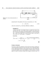
Heat transfer
Heat will be removed from the exposed surface of a semi-infinite region,
with a b.c. of either the first or the third kind, in accordance with Fourier’s
law:
q =−k
∂T
∂x





x=0
=
k(T
∞
−T
i
)
√
αt
dΘ
dζ





ζ=0
Differentiating Θ as given by eqn. (5.50), we obtain, for the b.c. of the
first kind,
q =
k(T
∞
−T
i
)
√
αt


1
√
π
e
−ζ
2
/4

ζ=0
=
k(T
∞
−T
i
)
√
παt
(5.54)
Thus, q decreases with increasing time, as t
−1/2
. When the temperature
of the surface is first changed, the heat removal rate is enormous. Then
it drops off rapidly.
It often occurs that we suddenly apply a specified input heat flux,
q
w
, at the boundary of a semi-infinite region. In such a case, we can
§5.6 Transient heat conduction to a semi-infinite region 229
differentiate the heat diffusion equation with respect to x,so
α

∂
3
T
∂x
3
=
∂
2
T
∂t∂x
When we substitute q =−k∂T/∂x in this, we obtain
α
∂
2
q
∂x
2
=
∂q
∂t
with the b.c.’s:
q(x = 0,t >0) = q
w
or
q
w
−q
q
w






x=0
= 0
q(x  0,t = 0) = 0or
q
w
−q
q
w





t=0
= 1
What we have done here is quite elegant. We have made the problem
of predicting the local heat flux q into exactly the same form as that of
predicting the local temperature in a semi-infinite region subjected to a
step change of wall temperature. Therefore, the solution must be the
same:
q
w
−q
q
w
= erf


x
2
√
αt

. (5.55)
The temperature distribution is obtained by integrating Fourier’s law. At
the wall, for example:

T
w
T
i
dT =−

0
∞
q
k
dx
where T
i
= T(x →∞) and T
w
= T(x = 0). Then
T
w
= T
i

+
q
w
k

∞
0
erfc(x/2

αt) dx
This becomes
T
w
= T
i
+
q
w
k

αt

∞
0
erfc(ζ/2)dζ

 
=2/
√
π

so
T
w
(t) = T
i
+2
q
w
k

αt
π
(5.56)
230 Transient and multidimensional heat conduction §5.6
Figure 5.17 A bubble growing in a
superheated liquid.
Example 5.6 Predicting the Growth Rate of a Vapor Bubble
in an Infinite Superheated Liquid
This prediction is relevant to a large variety of processes, ranging
from nuclear thermodynamics to the direct-contact heat exchange. It
was originally presented by Max Jakob and others in the early 1930s
(see, e.g., [5.10, Chap. I]). Jakob (pronounced Yah

-kob) was an im-
portant figure in heat transfer during the 1920s and 1930s. He left
Nazi Germany in 1936 to come to the United States. We encounter
his name again later.
Figure 5.17 shows how growth occurs. When a liquid is super-
heated to a temperature somewhat above its boiling point, a small
gas or vapor cavity in that liquid will grow. (That is what happens in

the superheated water at the bottom of a teakettle.)
This bubble grows into the surrounding liquid because its bound-
ary is kept at the saturation temperature, T
sat
, by the near-equilibrium
coexistence of liquid and vapor. Therefore, heat must flow from the
superheated surroundings to the interface, where evaporation occurs.
So long as the layer of cooled liquid is thin, we should not suffer too
much error by using the one-dimensional semi-infinite region solu-
tion to predict the heat flow.
§5.6 Transient heat conduction to a semi-infinite region 231
Thus, we can write the energy balance at the bubble interface:

−q
W
m
2


4πR
2
m
2


 
Q into bubble
=

ρ

g
h
fg
J
m
3


dV
dt
m
3
s


 
rate of energy increase
of the bubble
and then substitute eqn. (5.54) for q and 4πR
3
/3 for the volume, V.
This gives
k(T
sup
−T
sat
)
√
απt
= ρ

g
h
fg
dR
dt
(5.57)
Integrating eqn. (5.57) from R = 0att = 0uptoR at t, we obtain
Jakob’s prediction:
R =
2
√
π
k∆T
ρ
g
h
fg
√
α

t (5.58)
This analysis was done without assuming the curved bubble interface
to be plane, 24 years after Jakob’s work, by Plesset and Zwick [5.11]. It
was verified in a more exact way after another 5 years by Scriven [5.12].
These calculations are more complicated, but they lead to a very similar
result:
R =
2
√
3

√
π
k∆T
ρ
g
h
fg
√
α

t =
√
3 R
Jakob
. (5.59)
Both predictions are compared with some of the data of Dergarabe-
dian [5.13] in Fig. 5.18. The data and the exact theory match almost
perfectly. The simple theory of Jakob et al. shows the correct depen-
dence on R on all its variables, but it shows growth rates that are low
by a factor of
√
3. This is because the expansion of the spherical bub-
ble causes a relative motion of liquid toward the bubble surface, which
helps to thin the region of thermal influence in the radial direction. Con-
sequently, the temperature gradient and heat transfer rate are higher
than in Jakob’s model, which neglected the liquid motion. Therefore, the
temperature profile flattens out more slowly than Jakob predicts, and the
bubble grows more rapidly.
Experiment 5.2
Touch various objects in the room around you: glass, wood, cork-

board, paper, steel, and gold or diamond, if available. Rank them in
232 Transient and multidimensional heat conduction §5.6
Figure 5.18 The growth of a vapor bubble—predictions and
measurements.
order of which feels coldest at the first instant of contact (see Problem
5.29).
The more advanced theory of heat conduction (see, e.g., [5.6]) shows
that if two semi-infinite regions at uniform temperatures T
1
and T
2
are
placed together suddenly, their interface temperature, T
s
, is given by
6
T
s
−T
2
T
1
−T
2
=

(kρc
p
)
2


(kρc
p
)
1
+

(kρc
p
)
2
If we identify one region with your body (T
1
 37
◦
C) and the other with
the object being touched (T
2
 20
◦
C), we can determine the temperature,
T
s
, that the surface of your finger will reach upon contact. Compare
the ranking you obtain experimentally with the ranking given by this
equation.
Notice that your bloodstream and capillary system provide a heat
6
For semi-infinite regions, initially at uniform temperatures, T
s

does not vary with
time. For finite bodies, T
s
will eventually change. A constant value of T
s
means that
each of the two bodies independently behaves as a semi-infinite body whose surface
temperature has been changed to T
s
at time zero. Consequently, our previous results—
eqns. (5.50), (5.51), and (5.54)—apply to each of these bodies while they may be treated
as semi-infinite. We need only replace T
∞
by T
s
in those equations.
§5.6 Transient heat conduction to a semi-infinite region 233
source in your finger, so the equation is valid only for a moment. Then
you start replacing heat lost to the objects. If you included a diamond
among the objects that you touched, you will notice that it warmed up
almost instantly. Most diamonds are quite small but are possessed of the
highest known value of α. Therefore, they can behave as a semi-infinite
region only for an instant, and they usually feel warm to the touch.
Conduction to a semi-infinite region with a harmonically
oscillating temperature at the boundary
Suppose that we approximate the annual variation of the ambient tem-
perature as sinusoidal and then ask what the influence of this variation
will be beneath the ground. We want to calculate T −
T (where
T is the

time-average surface temperature) as a function of: depth, x; thermal
diffusivity, α; frequency of oscillation, ω; amplitude of oscillation, ∆T ;
and time, t. There are six variables in K, m, and s, so the problem can be
represented in three dimensionless variables:
Θ ≡
T −
T
∆T
; Ω ≡ ωt; ξ ≡ x

ω
2α
.
We pose the problem as follows in these variables. The heat conduc-
tion equation is
1
2
∂
2
Θ
∂ξ
2
=
∂Θ
∂Ω
(5.60)
and the b.c.’s are
Θ




ξ=0
= cos ωt and Θ



ξ>0
= finite (5.61)
No i.c. is needed because, after the initial transient decays, the remaining
steady oscillation must be periodic.
The solution is given by Carslaw and Jaeger (see [5.6, §2.6] or work
Problem 5.16). It is
Θ
(
ξ,Ω
)
= e
−ξ
cos
(
Ω − ξ
)
(5.62)
This result is plotted in Fig. 5.19. It shows that the surface temperature
variation decays exponentially into the region and suffers a phase shift
as it does so.
234 Transient and multidimensional heat conduction §5.6
Figure 5.19 The temperature variation within a semi-infinite
region whose temperature varies harmonically at the boundary.
Example 5.7

How deep in the earth must we dig to find the temperature wave that
was launched by the coldest part of the last winter if it is now high
summer?
Solution. ω = 2π rad/yr, and Ω = ωt = 0 at the present. First,
we must find the depths at which the Ω = 0 curve reaches its lo-
cal extrema. (We pick the Ω = 0 curve because it gives the highest
temperature at t = 0.)
dΘ
dξ





Ω=0
=−e
−ξ
cos(0 −ξ) + e
−ξ
sin(0 −ξ) = 0
This gives
tan(0 −ξ) = 1soξ =
3π
4
,
7π
4
,
and the first minimum occurs where ξ = 3π/4 = 2.356, as we can see
in Fig. 5.19. Thus,

ξ = x

ω/2α = 2.356
§5.7 Steady multidimensional heat conduction 235
or, if we take α = 0.139×10
−6
m
2
/s (given in [5.14] for coarse, gravelly
earth),
x = 2.356


2π
2

0.139 ×10
−6

1
365(24)(3600)
= 2.783 m
If we dug in the earth, we would find it growing older and colder until
it reached a maximum coldness at a depth of about 2.8 m. Farther
down, it would begin to warm up again, but not much. In midwinter
(Ω = π), the reverse would be true.
5.7 Steady multidimensional heat conduction
Introduction
The general equation for T(


r) during steady conduction in a region of
constant thermal conductivity, without heat sources, is called Laplace’s
equation:
∇
2
T = 0 (5.63)
It looks easier to solve than it is, since [recall eqn. (2.12) and eqn. (2.14)]
the Laplacian, ∇
2
T , is a sum of several second partial derivatives. We
solved one two-dimensional heat conduction problem in Example 4.1,
but this was not difficult because the boundary conditions were made to
order. Depending upon your mathematical background and the specific
problem, the analytical solution of multidimensional problems can be
anything from straightforward calculation to a considerable challenge.
The reader who wishes to study such analyses in depth should refer to
[5.6]or[5.15], where such calculations are discussed in detail.
Faced with a steady multidimensional problem, three routes are open
to us:
• Find out whether or not the analytical solution is already available
in a heat conduction text or in other published literature.
• Solve the problem.
(a) Analytically.
(b) Numerically.
• Obtain the solution graphically if the problem is two-dimensional.
It is to the last of these options that we give our attention next.
236 Transient and multidimensional heat conduction §5.7
Figure 5.20 The two-dimensional flow
of heat between two isothermal walls.
The flux plot

The method of flux plotting will solve all steady planar problems in which
all boundaries are held at either of two temperatures or are insulated.
With a little skill, it will provide accuracies of a few percent. This accuracy
is almost always greater than the accuracy with which the b.c.’s and k
can be specified; and it displays the physical sense of the problem very
clearly.
Figure 5.20 shows heat flowing from one isothermal wall to another
in a regime that does not conform to any convenient coordinate scheme.
We identify a series of channels, each which carries the same heat flow,
δQ W/m. We also include a set of equally spaced isotherms, δT apart,
between the walls. Since the heat fluxes in all channels are the same,



δQ



= k
δT
δn
δs (5.64)
Notice that if we arrange things so that δQ, δT , and k are the same
for flow through each rectangle in the flow field, then δs/δn must be the
same for each rectangle. We therefore arbitrarily set the ratio equal to
unity, so all the elements appear as distorted squares.
The objective then is to sketch the isothermal lines and the adiabatic,
7
7
These are lines in the direction of heat flow. It immediately follows that there can

§5.7 Steady multidimensional heat conduction 237
or heat flow, lines which run perpendicular to them. This sketch is to be
done subject to two constraints
• Isothermal and adiabatic lines must intersect at right angles.
• They must subdivide the flow field into elements that are nearly
square—“nearly” because they have slightly curved sides.
Once the grid has been sketched, the temperature anywhere in the field
can be read directly from the sketch. And the heat flow per unit depth
into the paper is
Q W/m = NkδT
δs
δn
=
N
I
k∆T
(5.65)
where N is the number of heat flow channels and I is the number of
temperature increments, ∆T /δT.
The first step in constructing a flux plot is to draw the boundaries of
the region accurately in ink, using either drafting software or a straight-
edge. The next is to obtain a soft pencil (such as a no. 2 grade) and a
soft eraser. We begin with an example that was executed nicely in the
influential Heat Transfer Notes [5.3] of the mid-twentieth century. This
example is shown in Fig. 5.21.
The particular example happens to have an axis of symmetry in it. We
immediately interpret this as an adiabatic boundary because heat cannot
cross it. The problem therefore reduces to the simpler one of sketching
lines in only one half of the area. We illustrate this process in four steps.
Notice the following steps and features in this plot:

• Begin by dividing the region, by sketching in either a single isother-
mal or adiabatic line.
• Fill in the lines perpendicular to the original line so as to make
squares. Allow the original line to move in such a way as to accom-
modate squares. This will always require some erasing. Therefore:
• Never make the original lines dark and firm.
• By successive subdividing of the squares, make the final grid. Do
not make the grid very fine. If you do, you will lose accuracy because
the lack of perpendicularity and squareness will be less evident to
the eye. Step IV in Fig. 5.21 is as fine a grid as should ever be made.
be no component of heat flow normal to them; they must be adiabatic.
Figure 5.21 The evolution of a flux plot.
238