A HEAT TRANSFER TEXTBOOK - THIRD EDITION Episode 2 Part 1 doc

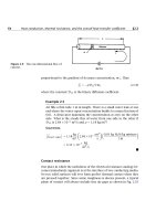
§5.7 Steady multidimensional heat conduction 239
• If you have doubts about whether any large, ill-shaped regions are
correct, fill them in with an extra isotherm and adiabatic line to
be sure that they resolve into appropriate squares (see the dashed
lines in Fig. 5.21).
• Fill in the final grid, when you are sure of it, either in hard pencil or
pen, and erase any lingering background sketch lines.
• Your flow channels need not come out even. Notice that there is an
extra 1/7 of a channel in Fig. 5.21. This is simply counted as 1/7of
a square in eqn. (5.65).
• Never allow isotherms or adiabatic lines to intersect themselves.
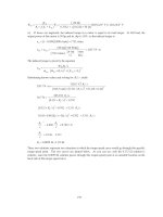
When the sketch is complete, we can return to eqn. (5.65) to compute
the heat flux. In this case
Q =
N
I
k∆T =
2(6.14)
4
k∆T = 3.07 k∆T
When the authors of [5.3] did this problem, they obtained N/I = 3.00—a
value only 2% below ours. This kind of agreement is typical when flux
plotting is done with care.
Figure 5.22 A flux plot with no axis of symmetry to guide
construction.
240 Transient and multidimensional heat conduction §5.7
One must be careful not to grasp at a false axis of symmetry. Figure
5.22 shows a shape similar to the one that we just treated, but with un-
equal legs. In this case, no lines must enter (or leave) the corners A and
B. The reason is that since there is no symmetry, we have no guidance
as to the direction of the lines at these corners. In particular, we know

that a line leaving A will no longer arrive at B.
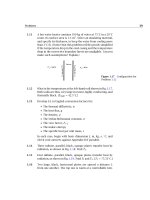
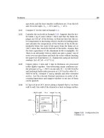
Example 5.8
A structure consists of metal walls, 8 cm apart, with insulating ma-
terial (k = 0.12 W/m·K) between. Ribs 4 cm long protrude from one
wall every 14 cm. They can be assumed to stay at the temperature of
that wall. Find the heat flux through the wall if the first wall is at 40
◦
C
and the one with ribs is at 0
◦
C. Find the temperature in the middle of
the wall, 2 cm from a rib, as well.
Figure 5.23 Heat transfer through a wall with isothermal ribs.
§5.7 Steady multidimensional heat conduction 241
Solution. The flux plot for this configuration is shown in Fig. 5.23.
For a typical section, there are approximately 5.6 isothermal incre-
ments and 6.15 heat flow channels, so
Q =
N
I
k∆T =
2(6.15)
5.6
(0.12)(40 − 0) = 10.54 W/m
where the factor of 2 accounts for the fact that there are two halves
in the section. We deduce the temperature for the point of interest,
A, by a simple proportionality:
T
point A
=

2.1
5.6
(40 − 0) = 15
◦
C
The shape factor
A heat conduction shape factor S may be defined for steady problems
involving two isothermal surfaces as follows:
Q ≡ Sk∆T. (5.66)
Thus far, every steady heat conduction problem we have done has taken
this form. For these situations, the heat flow always equals a function of
the geometric shape of the body multiplied by k∆T .
The shape factor can be obtained analytically, numerically, or through
flux plotting. For example, let us compare eqn. (5.65) and eqn. (5.66):
Q
W
m
= (S dimensionless)

k∆T
W
m

=
N
I
k∆T (5.67)
This shows S to be dimensionless in a two-dimensional problem, but in
three dimensions S has units of meters:
Q W = (S m)


k∆T
W
m

. (5.68)
It also follows that the thermal resistance of a two-dimensional body is
R
t
=
1
kS
where Q =
∆T
R
t
(5.69)
For a three-dimensional body, eqn. (5.69) is unchanged except that the
dimensions of Q and R
t
differ.
8
8
Recall that we noted after eqn. (2.22) that the dimensions of R
t
changed, depending
on whether or not Q was expressed in a unit-length basis.
242 Transient and multidimensional heat conduction §5.7
Figure 5.24 The shape factor for two similar bodies of differ-
ent size.

The virtue of the shape factor is that it summarizes a heat conduction
solution in a given configuration. Once S is known, it can be used again
and again. That S is nondimensional in two-dimensional configurations
means that Q is independent of the size of the body. Thus, in Fig. 5.21, S
is always 3.07—regardless of the size of the figure—and in Example 5.8, S
is 2(6.15)/5.6 = 2.196, whether or not the wall is made larger or smaller.
When a body’s breadth is increased so as to increase Q, its thickness in
the direction of heat flow is also increased so as to decrease Q by the
same factor.
Example 5.9
Calculate the shape factor for a one-quarter section of a thick cylinder.
Solution. We already know R
t
for a thick cylinder. It is given by
eqn. (2.22). From it we compute
S
cyl
=
1
kR
t
=
2π
ln(r
o
/r
i
)
so on the case of a quarter-cylinder,
S =

π
2ln(r
o
/r
i
)
The quarter-cylinder is pictured in Fig. 5.24 for a radius ratio, r
o
/r
i
=
3, but for two different sizes. In both cases S = 1.43. (Note that the
same S is also given by the flux plot shown.)
§5.7 Steady multidimensional heat conduction 243
Figure 5.25 Heat transfer through a
thick, hollow sphere.
Example 5.10
Calculate S for a thick hollow sphere, as shown in Fig. 5.25.
Solution. The general solution of the heat diffusion equation in
spherical coordinates for purely radial heat flow is:
T =
C
1
r
+C
2
when T = fn(r only). The b.c.’s are
T
(
r = r

i
)
= T
i
and T
(
r = r
o
)
= T
o
substituting the general solution in the b.c.’s we get
C
1
r
i
+C
2
= T
i
and
C
1
r
o
+C
1
= T
o
Therefore,

C
1
=
T
i
−T
o
r
o
−r
i
r
i
r
o
and C
2
= T
i
−
T
i
−T
o
r
o
−r
i
r
o

Putting C
1
and C
2
in the general solution, and calling T
i
− T
o
≡ ∆T ,
we get
T = T
i
+∆T

r
i
r
o
r(r
o
−r
i
)
−
r
o
r
o
−r
i


Then
Q =−kA
dT
dr
=
4π(r
i
r
o
)
r
o
−r
i
k∆T
S =
4π(r
i
r
o
)
r
o
−r
i
m
where S now has the dimensions of m.
244 Transient and multidimensional heat conduction §5.7
Table 5.4 includes a number of analytically derived shape factors for

use in calculating the heat flux in different configurations. Notice that
these results will not give local temperatures. To obtain that information,
one must solve the Laplace equation, ∇
2
T = 0, by one of the methods
listed at the beginning of this section. Notice, too, that this table is re-
stricted to bodies with isothermal and insulated boundaries.
In the two-dimensional cases, both a hot and a cold surface must be
present in order to have a steady-state solution; if only a single hot (or
cold) body is present, steady state is never reached. For example, a hot
isothermal cylinder in a cooler, infinite medium never reaches steady
state with that medium. Likewise, in situations 5, 6, and 7 in the table,
the medium far from the isothermal plane must also be at temperature
T
2
in order for steady state to occur; otherwise the isothermal plane and
the medium below it would behave as an unsteady, semi-infinite body. Of
course, since no real medium is truly infinite, what this means in practice
is that steady state only occurs after the medium “at infinity” comes to
a temperature T
2
. Conversely, in three-dimensional situations (such as
4, 8, 12, and 13), a body can come to steady state with a surrounding
infinite or semi-infinite medium at a different temperature.
Example 5.11
A spherical heat source of 6 cm in diameter is buried 30 cm below the
surface of a very large box of soil and kept at 35
◦
C. The surface of
the soil is kept at 21

◦
C. If the steady heat transfer rate is 14 W, what
is the thermal conductivity of this sample of soil?
Solution.
Q = Sk∆T =

4πR
1 − R/2h

k∆T
where S is that for situation 7 in Table 5.4. Then
k =
14 W
(35 − 21)K
1 − (0.06/2)

2(0.3)
4π(0.06/2) m
= 2.545 W/m·K
Readers who desire a broader catalogue of shape factors should refer
to [5.16], [5.18], or [5.19].
Table 5.4 Conduction shape factors: Q = Sk∆T .
Situation Shape factor, S Dimensions Source
1. Conduction through a slab
A/L meter Example 2.2
2. Conduction through wall of a long
thick cylinder
2π
ln
(

r
o
/r
i
)
none Example 5.9
3. Conduction through a thick-walled
hollow sphere
4π
(
r
o
r
i
)
r
o
−r
i
meter Example 5.10
4. The boundary of a spherical hole of
radius R conducting into an infinite
medium
4πR meter
Problems 5.19
and 2.15
5. Cylinder of radius R and length L,
transferring heat to a parallel
isothermal plane; h  L
2πL

cosh
−1
(
h/R
)
meter [5.16]
6. Same as item 5, but with L →∞
(two-dimensional conduction)
2π
cosh
−1
(
h/R
)
none [5.16]
7. An isothermal sphere of radius R
transfers heat to an isothermal
plane; R/h < 0.8 (see item 4)
4πR
1 −R/2h
meter [5.16, 5.17]
245
Table 5.4 Conduction shape factors: Q = Sk∆T (con’t).
Situation Shape factor, S Dimensions Source
8. An isothermal sphere of radius R,
near an insulated plane, transfers
heat to a semi-infinite medium at
T
∞
(see items 4 and 7)

4πR
1 +R/2h
meter [5.18]
9. Parallel cylinders exchange heat in
an infinite conducting medium
2π
cosh
−1

L
2
−R
2
1
−R
2
2
2R
1
R
2

none [5.6]
10. Same as 9, but with cylinders
widely spaced; L  R
1
and R
2
2π
cosh

−1

L
2R
1

+cosh
−1

L
2R
2

none [5.16]
11. Cylinder of radius R
i
surrounded
by eccentric cylinder of radius
R
o
>R
i
; centerlines a distance L
apart (see item 2)
2π
cosh
−1

R
2

o
+R
2
i
−L
2
2R
o
R
i

none [5.6]
12. Isothermal disc of radius R on an
otherwise insulated plane conducts
heat into a semi-infinite medium at
T
∞
below it
4R meter [5.6]
13. Isothermal ellipsoid of semimajor
axis b and semiminor axes a
conducts heat into an infinite
medium at T
∞
; b>a(see 4)
4πb

1 −a
2


b
2
tanh
−1


1 −a
2

b
2

meter [5.16]
246
§5.8 Transient multidimensional heat conduction 247
Figure 5.26 Resistance vanishes where
two isothermal boundaries intersect.
The problem of locally vanishing resistance
Suppose that two different temperatures are specified on adjacent sides
of a square, as shown in Fig. 5.26. The shape factor in this case is
S =
N
I
=
∞
4
=∞
(It is futile to try and count channels beyond N  10, but it is clear that
they multiply without limit in the lower left corner.) The problem is that
we have violated our rule that isotherms cannot intersect and have cre-

ated a 1/r singularity. If we actually tried to sustain such a situation,
the figure would be correct at some distance from the corner. However,
where the isotherms are close to one another, they will necessarily influ-
ence and distort one another in such a way as to avoid intersecting. And
S will never really be infinite, as it appears to be in the figure.
5.8 Transient multidimensional heat conduction—
The tactic of superposition
Consider the cooling of a stubby cylinder, such as the one shown in
Fig. 5.27a. The cylinder is initially at T = T
i
, and it is suddenly sub-
jected to a common b.c. on all sides. It has a length 2L and a radius r
o
.
Finding the temperature field in this situation is inherently complicated.
248 Transient and multidimensional heat conduction §5.8
It requires solving the heat conduction equation for T = fn(r,z,t) with
b.c.’s of the first, second, or third kind.
However, Fig. 5.27a suggests that this can somehow be viewed as a
combination of an infinite cylinder and an infinite slab. It turns out that
the problem can be analyzed from that point of view.
If the body is subject to uniform b.c.’s of the first, second, or third
kind, and if it has a uniform initial temperature, then its temperature
response is simply the product of an infinite slab solution and an infinite
cylinder solution each having the same boundary and initial conditions.
For the case shown in Fig. 5.27a, if the cylinder begins convective cool-
ing into a medium at temperature T
∞
at time t = 0, the dimensional
temperature response is

T
(
r,z,t
)
−T
∞
=

T
slab
(z, t) −T
∞

×

T
cyl
(r , t) −T
∞

(5.70a)
Observe that the slab has as a characteristic length L, its half thickness,
while the cylinder has as its characteristic length R, its radius. In dimen-
sionless form, we may write eqn. (5.70a)as
Θ ≡
T(r,z,t)−T
∞
T
i
−T

∞
=

Θ
inf slab
(ξ, Fo
s
, Bi
s
)

Θ
inf cyl
(ρ, Fo
c
, Bi
c
)

(5.70b)
For the cylindrical component of the solution,
ρ =
r
r
o
, Fo
c
=
αt
r

2
o
, and Bi
c
=
hr
o
k
,
while for the slab component of the solution
ξ =
z
L
+1, Fo
s
=
αt
L
2
, and Bi
s
=
hL
k
.
The component solutions are none other than those discussed in Sec-
tions 5.3–5.5. The proof of the legitimacy of such product solutions is
given by Carlsaw and Jaeger [5.6, §1.15].
Figure 5.27b shows a point inside a one-eighth-infinite region, near the
corner. This case may be regarded as the product of three semi-infinite

bodies. To find the temperature at this point we write
Θ ≡
T(x
1
,x
2
,x
3
,t)−T
∞
T
i
−T
∞
=
[
Θ
semi
(ζ
1
,β)
][
Θ
semi
(ζ
2
,β)
][
Θ
semi

(ζ
3
,β)
]
(5.71)
Figure 5.27 Various solid bodies whose transient cooling can
be treated as the product of one-dimensional solutions.
249
250 Transient and multidimensional heat conduction §5.8
in which Θ
semi
is either the semi-infinite body solution given by eqn. (5.53)
when convection is present at the boundary or the solution given by
eqn. (5.50) when the boundary temperature itself is changed at time zero.
Several other geometries can also be represented by product solu-
tions. Note that for of these solutions, the value of Θ at t = 0 is one for
each factor in the product.
Example 5.12
A very long 4 cm square iron rod at T
i
= 100
◦
C is suddenly immersed
in a coolant at T
∞
= 20
◦
C with h = 800 W/m
2
K. What is the temper-

ature on a line 1 cm from one side and 2 cm from the adjoining side,
after 10 s?
Solution. With reference to Fig. 5.27c, see that the bar may be
treated as the product of two slabs, each 4 cm thick. We first evaluate
Fo
1
= Fo
2
= αt/L
2
= (0.0000226 m
2
/s)(10 s)

(0.04 m/2)
2
= 0.565,
and Bi
1
= Bi
2
= hL

k = 800(0.04/2)/76 = 0.2105, and we then
write
Θ

x
L


1
= 0,

x
L

2
=
1
2
, Fo
1
, Fo
2
, Bi
−1
1
, Bi
−1
2

= Θ
1

x
L

1
= 0, Fo
1

= 0.565, Bi
−1
1
= 4.75


 
= 0.93 from upper left-hand
side of Fig. 5.7
×Θ
2

x
L

2
=
1
2
, Fo
2
= 0.565, Bi
−1
2
= 4.75


 
= 0.91 from interpolation
between lower lefthand side and

upper righthand side of Fig. 5.7
Thus, at the axial line of interest,
Θ = (0.93)(0.91) = 0.846
so
T −20
100 − 20
= 0.846 or T = 87.7
◦
C
Transient multidimensional heat conduction 251
Product solutions can also be used to determine the mean tempera-
ture,
Θ, and the total heat removal, Φ, from a multidimensional object.
For example, when two or three solutions (Θ
1
, Θ
2
, and perhaps Θ
3
) are
multiplied to obtain Θ, the corresponding mean temperature of the mul-
tidimensional object is simply the product of the one-dimensional mean
temperatures from eqn. (5.40)
Θ = Θ
1
(
Fo
1
, Bi
1

)
×
Θ
2
(
Fo
2
, Bi
2
)
for two factors (5.72a)
Θ = Θ
1
(
Fo
1
, Bi
1
)
×
Θ
2
(
Fo
2
, Bi
2
)
×Θ
3

(
Fo
3
, Bi
3
)
for three factors.
(5.72b)
Since Φ = 1 −
Θ, a simple calculation shows that Φ can found from Φ
1
,
Φ
2
, and Φ
3
as follows:
Φ = Φ
1
+Φ
2
(
1 − Φ
1
)
for two factors (5.73a)
Φ = Φ
1
+Φ
2

(
1 − Φ
1
)
+Φ
3
(
1 − Φ
2
)(
1 − Φ
1
)
for three factors. (5.73b)
Example 5.13
For the bar described in Example 5.12, what is the mean temperature
after 10 s and how much heat has been lost at that time?
Solution. For the Biot and Fourier numbers given in Example 5.12,
we find from Fig. 5.10a
Φ
1
(
Fo
1
= 0.565, Bi
1
= 0.2105
)
= 0.10
Φ

2
(
Fo
2
= 0.565, Bi
2
= 0.2105
)
= 0.10
and, with eqn. (5.73a),
Φ = Φ
1
+Φ
2
(
1 − Φ
1
)
= 0.19
The mean temperature is
Θ =
T −20
100 − 20
= 1 −Φ = 0.81
so
T = 20 + 80(0.81) = 84.8
◦
C
252 Chapter 5: Transient and multidimensional heat conduction
Problems

5.1 Rework Example 5.1, and replot the solution, with one change.
This time, insert the thermometer at zero time, at an initial
temperature <(T
i
−bT ).
5.2 A body of known volume and surface area and temperature T
i
is suddenly immersed in a bath whose temperature is rising
as T
bath
= T
i
+ (T
0
− T
i
)e
t/τ
. Let us suppose that h is known,
that τ = 10ρcV/
hA, and that t is measured from the time of
immersion. The Biot number of the body is small. Find the
temperature response of the body. Plot the response and the
bath temperature as a function of time up to t = 2τ. (Do not
use Laplace transform methods except, perhaps, as a check.)
5.3 A body of known volume and surface area is immersed in
a bath whose temperature is varying sinusoidally with a fre-
quency ω about an average value. The heat transfer coefficient
is known and the Biot number is small. Find the temperature
variation of the body after a long time has passed, and plot it

along with the bath temperature. Comment on any interesting
aspects of the solution.
A suggested program for solving this problem:
• Write the differential equation of response.
• To get the particular integral of the complete equation,
guess that T −T
mean
= C
1
cos ωt +C
2
sin ωt. Substitute
this in the differential equation and find C
1
and C
2
values
that will make the resulting equation valid.
• Write the general solution of the complete equation. It
will have one unknown constant in it.
• Write any initial condition you wish—the simplest one you
can think of—and use it to get rid of the constant.
• Let the time be large and note which terms vanish from
the solution. Throw them away.
• Combine two trigonometric terms in the solution into a
term involving sin(ωt − β), where β = fn(ωT ) is the
phase lag of the body temperature.
5.4 A block of copper floats within a large region of well-stirred
mercury. The system is initially at a uniform temperature, T
i

.
Problems 253
There is a heat transfer coefficient, h
m
, on the inside of the thin
metal container of the mercury and another one,
h
c
, between
the copper block and the mercury. The container is then sud-
denly subjected to a change in ambient temperature from T
i
to
T
s
<T
i
. Predict the temperature response of the copper block,
neglecting the internal resistance of both the copper and the
mercury. Check your result by seeing that it fits both initial
conditions and that it gives the expected behavior at t →∞.
5.5 Sketch the electrical circuit that is analogous to the second-
order lumped capacity system treated in the context of Fig. 5.5
and explain it fully.
5.6 A one-inch diameter copper sphere with a thermocouple in
its center is mounted as shown in Fig. 5.28 and immersed in
water that is saturated at 211
◦
F. The figure shows the ther-
mocouple reading as a function of time during the quench-

ing process. If the Biot number is small, the center temper-
ature can be interpreted as the uniform temperature of the
sphere during the quench. First draw tangents to the curve,
and graphically differentiate it. Then use the resulting values
of dT /dt to construct a graph of the heat transfer coefficient
as a function of (T
sphere
− T
sat
). The result will give actual
values of
h during boiling over the range of temperature dif-
ferences. Check to see whether or not the largest value of the
Biot number is too great to permit the use of lumped-capacity
methods.
5.7 A butt-welded 36-gage thermocouple is placed in a gas flow
whose temperature rises at the rate 20
◦
C/s. The thermocou-
ple steadily records a temperature 2.4
◦
C below the known gas
flow temperature. If ρc is 3800 kJ/m
3
K for the thermocouple
material, what is
h on the thermocouple? [h = 1006 W/m
2
K.]
5.8 Check the point on Fig. 5.7 at Fo = 0.2, Bi = 10, and x/L = 0

analytically.
5.9 Prove that when Bi is large, eqn. (5.34) reduces to eqn. (5.33).
5.10 Check the point at Bi = 0.1 and Fo = 2.5 on the slab curve in
Fig. 5.10 analytically.
254 Chapter 5: Transient and multidimensional heat conduction
Figure 5.28 Configuration and temperature response for
Problem 5.6
5.11 Sketch one of the curves in Fig. 5.7, 5.8,or5.9 and identify:
• The region in which b.c.’s of the third kind can be replaced
with b.c.’s of the first kind.
• The region in which a lumped-capacity response can be
assumed.
• The region in which the solid can be viewed as a semi-
infinite region.
5.12 Water flows over a flat slab of Nichrome, 0.05 mm thick, which
serves as a resistance heater using AC power. The apparent
value of
h is 2000 W/m
2
K. How much surface temperature
fluctuation will there be?
Problems 255
5.13 Put Jakob’s bubble growth formula in dimensionless form, iden-
tifying a “Jakob number”, Ja ≡ c
p
(T
sup
− T
sat
)/h

fg
as one of
the groups. (Ja is the ratio of sensible heat to latent heat.) Be
certain that your nondimensionalization is consistent with the
Buckingham pi-theorem.
5.14 A 7 cm long vertical glass tube is filled with water that is uni-
formly at a temperature of T = 102
◦
C. The top is suddenly
opened to the air at 1 atm pressure. Plot the decrease of the
height of water in the tube by evaporation as a function of time
until the bottom of the tube has cooled by 0.05
◦
C.
5.15 A slab is cooled convectively on both sides from a known ini-
tial temperature. Compare the variation of surface tempera-
ture with time as given in Fig. 5.7 with that given by eqn. (5.53)
if Bi = 2. Discuss the meaning of your comparisons.
5.16 To obtain eqn. (5.62), assume a complex solution of the type
Θ = fn(ξ)exp(iΩ), where i ≡
√
−1. This will assure that the
real part of your solution has the required periodicity and,
when you substitute it in eqn. (5.60), you will get an easy-to-
solve ordinary d.e. in fn(ξ).
5.17 A certain steel cylinder wall is subjected to a temperature os-
cillation that we approximate at T = 650
◦
C +(300
◦

C) cos ωt,
where the piston fires eight times per second. For stress de-
sign purposes, plot the amplitude of the temperature variation
in the steel as a function of depth. If the cylinder is 1 cm thick,
can we view it as having infinite depth?
5.18 A 40 cm diameter pipe at 75
◦
C is buried in a large block of
Portland cement. It runs parallel with a 15
◦
C isothermal sur-
face at a depth of 1 m. Plot the temperature distribution along
the line normal to the 15
◦
C surface that passes through the
center of the pipe. Compute the heat loss from the pipe both
graphically and analytically.
5.19 Derive shape factor 4 in Table 5.4.
5.20 Verify shape factor 9 in Table 5.4 with a flux plot. Use R
1
/R
2
=
2 and R
1
/L = ½. (Be sure to start out with enough blank paper
surrounding the cylinders.)
256 Chapter 5: Transient and multidimensional heat conduction
5.21 A copper block 1 in. thick and 3 in. square is held at 100
◦

F
on one 1 in. by 3 in. surface. The opposing 1 in. by 3 in.
surface is adiabatic for 2 in. and 90
◦
F for 1 inch. The re-
maining surfaces are adiabatic. Find the rate of heat transfer.
[Q = 36.8 W.]
5.22 Obtain the shape factor for any or all of the situations pic-
tured in Fig. 5.29a through j on pages 258–259. In each case,
present a well-drawn flux plot. [S
b
 1.03, S
c
 S
d
, S
g
=
1.]
5.23 Two copper slabs, 3 cm thick and insulated on the outside, are
suddenly slapped tightly together. The one on the left side is
initially at 100
◦
C and the one on the right side at 0
◦
C. Deter-
mine the left-hand adiabatic boundary’s temperature after 2.3
s have elapsed. [T
wall
 80.5

◦
C]
5.24 Estimate the time required to hard-cook an egg if:
Eggs cook as their
proteins denature and
coagulate. The time to
cook depends on
whether a soft or hard
cooked egg desired.
Eggs may be cooked by
placing them (cold or
warm) into cold water
before heating starts or
by placing warm eggs
directly into simmering
water [5.20].
• The minor diameter is 45 mm.
• k for the egg is about the same as for water. No signif-
icant heat release or change of properties occurs during
cooking.
•
h between the egg and the water is 140 W/m
2
K.
• The egg is put in boiling water when the egg is at a uni-
form temperature of 20
◦
C.
• The egg is done when the center reaches 75
◦

C.
5.25 Prove that T
1
in Fig. 5.5 cannot oscillate.
5.26 Show that when isothermal and adiabatic lines are interchanged
in a two-dimenisonal body, the new shape factor is the inverse
of the original one.
5.27 A 0.5 cm diameter cylinder at 300
◦
C is suddenly immersed
in saturated water at 1 atm. If
h = 10, 000 W/m
2
K, find the
centerline and surface temperatures after 0.2 s:
a. If the cylinder is copper.
b. If the cylinder is Nichrome V. [T
sfc
 200
◦
C.]
c. If the cylinder is Nichrome V, obtain the most accurate
value of the temperatures after 0.04 s that you can.
Problems 257
5.28 A large, flat electrical resistance strip heater is fastened to a
firebrick wall, unformly at 15
◦
C. When it is suddenly turned on,
it releases heat at the uniform rate of 4000 W/m
2

. Plot the tem-
perature of the brick immediately under the heater as a func-
tion of time if the other side of the heater is insulated. What
is the heat flux at a depth of 1 cm when the surface reaches
200
◦
C.
5.29 Do Experiment 5.2 and submit a report on the results.
5.30 An approximately spherical container, 2 cm in diameter, con-
taining electronic equipment is placed in wet mineral soil with
its center 2 m below the surface. The soil surface is kept at 0
◦
C.
What is the maximum rate at which energy can be released by
the equipment if the surface of the sphere is not to exceed
30
◦
C?
5.31 A semi-infinite slab of ice at −10
◦
C is exposed to air at 15
◦
C
through a heat transfer coefficient of 10 W/m
2
K. What is the
initial rate of melting of ice in kg/m
2
s? What is the asymp-
totic rate of melting? Describe the melting process in phys-

ical terms. (The latent heat of fusion of ice, h
sf
= 333, 300
J/kg.)
5.32 One side of an insulating firebrick wall, 10 cm thick, initially
at 20
◦
C is exposed to 1000
◦
C flame through a heat transfer
coefficient of 230 W/m
2
K. How long will it be before the other
side is too hot to touch, say at 65
◦
C? (Estimate properties at
500
◦
C, and assume that h is quite low on the cool side.)
5.33 A particular lead bullet travels for 0.5 sec within a shock wave
that heats the air near the bullet to 300
◦
C. Approximate the
bullet as a cylinder 0.8 cm in diameter. What is its surface
temperature at impact if
h = 600 W/m
2
K and if the bullet was
initially at 20
◦

C? What is its center temperature?
5.34 A loaf of bread is removed from an oven at 125
◦
C and set on
the (insulating) counter to cool in a kitchen at 25
◦
C. The loaf
is 30 cm long, 15 cm high, and 12 cm wide. If k = 0.05 W/m·K
and α = 5 × 10
−7
m
2
/s for bread, and h = 10 W/m
2
K, when
will the hottest part of the loaf have cooled to 60
◦
C? [About 1
h 5 min.]
Figure 5.29 Configurations for Problem 5.22
258
Figure 5.29 Configurations for Problem 5.22 (con’t)
259
260 Chapter 5: Transient and multidimensional heat conduction
5.35 A lead cube, 50 cm on each side, is initially at 20
◦
C. The sur-
roundings are suddenly raised to 200
◦
C and h around the cube

is 272 W/m
2
K. Plot the cube temperature along a line from
the center to the middle of one face after 20 minutes have
elapsed.
5.36 A jet of clean water superheated to 150
◦
C issues from a 1/16
inch diameter sharp-edged orifice into air at 1 atm, moving at
27 m/s. The coefficient of contraction of the jet is 0.611. Evap-
oration at T = T
sat
begins immediately on the outside of the jet.
Plot the centerline temperature of the jet and T(r/r
o
= 0.6) as
functions of distance from the orifice up to about 5 m. Neglect
any axial conduction and any dynamic interactions between
the jet and the air.
5.37 A 3 cm thick slab of aluminum (initially at 50
◦
C) is slapped
tightly againsta5cmslab of copper (initially at 20
◦
C). The out-
sides are both insulated and the contact resistance is neglible.
What is the initial interfacial temperature? Estimate how long
the interface will keep its initial temperature.
5.38 A cylindrical underground gasoline tank, 2 m in diameter and
4 m long, is embedded in 10

◦
C soil with k = 0.8 W/m
2
K and
α = 1.3 × 10
−6
m
2
/s. water at 27
◦
C is injected into the tank
to test it for leaks. It is well-stirred with a submerged ½ kW
pump. We observe the water level in a 10 cm I.D. transparent
standpipe and measure its rate of rise and fall. What rate of
change of height will occur after one hour if there is no leak-
age? Will the level rise or fall? Neglect thermal expansion and
deformation of the tank, which should be complete by the time
the tank is filled.
5.39 A47
◦
C copper cylinder, 3 cm in diameter, is suddenly im-
mersed horizontally in water at 27
◦
C in a reduced gravity en-
vironment. Plot T
cyl
as a function of time if g = 0.76 m/s
2
and if h = [2.733 +10.448(∆T
◦

C)
1/6
]
2
W/m
2
K. (Do it numer-
ically if you cannot integrate the resulting equation analyti-
cally.)
5.40 The mechanical engineers at the University of Utah end spring
semester by roasting a pig and having a picnic. The pig is
roughly cylindrical and about 26 cm in diameter. It is roasted
Problems 261
over a propane flame, whose products have properties similar
to those of air, at 280
◦
C. The hot gas flows across the pig at
about 2 m/s. If the meat is cooked when it reaches 95
◦
C, and
if it is to be served at 2:00 pm, what time should cooking com-
mence? Assume Bi to be large, but note Problem 7.40. The pig
is initially at 25
◦
C.
5.41 People from cold northern climates know not to grasp metal
with their bare hands in subzero weather. A very slightly frosted
peice of, say, cast iron will stick to your hand like glue in, say,
−20
◦

C weather and might tear off patches of skin. Explain this
quantitatively.
5.42 A 4 cm diameter rod of type 304 stainless steel has a very
small hole down its center. The hole is clogged with wax that
has a melting point of 60
◦
C. The rod is at 20
◦
C. In an attempt
to free the hole, a workman swirls the end of the rod—and
about a meter of its length—in a tank of water at 80
◦
C. If h
is 688 W/m
2
K on both the end and the sides of the rod, plot
the depth of the melt front as a function of time up to say, 4
cm.
5.43 A cylindrical insulator contains a single, very thin electrical re-
sistor wire that runs along a line halfway between the center
and the outside. The wire liberates 480 W/m. The thermal con-
ductivity of the insulation is 3 W/m
2
K, and the outside perime-
ter is held at 20
◦
C. Develop a flux plot for the cross section,
considering carefully how the field should look in the neigh-
borhood of the point through which the wire passes. Evaluate
the temperature at the center of the insulation.

5.44 A long, 10 cm square copper bar is bounded by 260
◦
C gas flows
on two opposing sides. These flows impose heat transfer coef-
ficients of 46 W/m
2
K. The two intervening sides are cooled by
natural convection to water at 15
◦
C, with a heat transfer coef-
ficient of 30 W/m
2
K. What is the heat flow through the block
and the temperature at the center of the block? (This could
be a pretty complicated problem, but take the trouble to think
about Biot numbers before you begin.)
5.45 Lord Kelvin made an interesting estimate of the age of the earth
in 1864. He assumed that the earth originated as a mass of
262 Chapter 5: Transient and multidimensional heat conduction
molten rock at 4144 K (7000
◦
F) and that it had been cooled
by outer space at 0 K ever since. To do this, he assumed
that Bi for the earth is very large and that cooling had thus
far penetrated through only a relatively thin (one-dimensional)
layer. Using α
rock
= 1.18 ×10
−6
m/s

2
and the measured sur-
face temperature gradient of the earth,
1
27
◦
C/m, Find Kelvin’s
value of Earth’s age. (Kelvin’s result turns out to be much
less than the accepted value of 4 billion years. His calcula-
tion fails because internal heat generation by radioactive de-
cay of the material in the surface layer causes the surface
temperature gradient to be higher than it would otherwise
be.)
5.46 A pure aluminum cylinder, 4 cm diam. by 8 cm long, is ini-
tially at 300
◦
C. It is plunged into a liquid bath at 40
◦
C with
h = 500 W/m
2
K. Calculate the hottest and coldest tempera-
tures in the cylinder after one minute. Compare these results
with the lumped capacity calculation, and discuss the compar-
ison.
5.47 When Ivan cleaned his freezer, he accidentally put a large can
of frozen juice into the refrigerator. The juice can is 17.8 cm
tall and has an 8.9 cm I.D. The can was at −15
◦
C in the freezer,

but the refrigerator is at 4
◦
C. The can now lies on a shelf of
widely-spaced plastic rods, and air circulates freely over it.
Thermal interactions with the rods can be ignored. The ef-
fective heat transfer coefficient to the can (for simultaneous
convection and thermal radiation) is 8 W/m
2
K. The can has
a 1.0 mm thick cardboard skin with k = 0.2 W/m·K. The
frozen juice has approximately the same physical properties
as ice.
a. How important is the cardboard skin to the thermal re-
sponse of the juice? Justify your answer quantitatively.
b. If Ivan finds the can in the refrigerator 30 minutes after
putting it in, will the juice have begun to melt?
5.48 A cleaning crew accidentally switches off the heating system
in a warehouse one Friday night during the winter, just ahead
of the holidays. When the staff return two weeks later, the
warehouse is quite cold. In some sections, moisture that con-
Problems 263
densed has formed a layer of ice 1 to 2 mm thick on the con-
crete floor. The concrete floor is 25 cm thick and sits on com-
pacted earth. Both the slab and the ground below it are now
at 20
◦
F. The building operator turns on the heating system,
quickly warming the air to 60
◦
F. If the heat transfer coefficient

between the air and the floor is 15 W/m
2
K, how long will it take
for the ice to start melting? Take α
concr
= 7.0 ×10
−7
m
2
/s and
k
concr
= 1.4 W/m·K, and make justifiable approximations as
appropriate.
5.49 A thick wooden wall, initially at 25
◦
C, is made of fir. It is sud-
denly exposed to flames at 800
◦
C. If the effective heat transfer
coefficient for convection and radiation between the wall and
the flames is 80 W/m
2
K, how long will it take the wooden wall
to reach its ignition temperature of 430
◦
C?
5.50 Cold butter does not spread as well as warm butter. A small
tub of whipped butter bears a label suggesting that, before
use, it be allowed to warm up in room air for 30 minutes after

being removed from the refrigerator. The tub has a diame-
ter of 9.1 cm with a height of 5.6 cm, and the properties of
whipped butter are: k = 0.125 W/m·K, c
p
= 2520 J/kg·K, and
ρ = 620 kg/m
3
. Assume that the tub’s cardboard walls of-
fer negligible thermal resistance, that
h = 10 W/m
2
K outside
the tub. Negligible heat is gained through the low conductivity
lip around the bottom of the tub. If the refrigerator temper-
ature was 5
◦
C and the tub has warmed for 30 minutes in a
room at 20
◦
C, find: the temperature in the center of the but-
ter tub, the temperature around the edge of the top surface of
the butter, and the total energy (in J) absorbed by the butter
tub.
5.51 A two-dimensional, 90
◦
annular sector has an adiabatic inner
arc, r = r
i
, and an adiabatic outer arc, r = r
o

. The flat sur-
face along θ = 0 is isothermal at T
1
, and the flat surface along
θ = π/2 is isothermal at T
2
. Show that the shape factor is
S = (2/π) ln(r
o
/r
i
).
5.52 Suppose that T
∞
(t) is the time-dependent environmental tem-
perature surrounding a convectively-cooled, lumped object.