A HEAT TRANSFER TEXTBOOK - THIRD EDITION Episode 2 Part 3 pot
Bạn đang xem bản rút gọn của tài liệu. Xem và tải ngay bản đầy đủ của tài liệu tại đây (223.45 KB, 25 trang )
§6.2 Laminar incompressible boundary layer on a flat surface 289
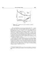
Figure 6.11 Comparison of the third-degree polynomial fit
with the exact b.l. velocity profile. (Notice that the approximate
result has been forced to u/u
∞
= 1 instead of 0.99 at y = δ.)
We integrate this using the b.c. δ
2
= 0atx = 0:
δ
2
=
280
13
νx
u
∞
or
δ
x
=
4.64
Re
x
(6.31)
This b.l. thickness is of the correct functional form, and the constant is
low by only 5.6%.
The skin friction coefficient
The fact that the function f (η) gives all information about flow in the b.l.
must be stressed. For example, the shear stress can be obtained from it
290 Laminar and turbulent boundary layers §6.2
by using Newton’s law of viscous shear:
τ
w
=µ
∂u
∂y
y=0
= µ
∂
∂y
u
∞
f
y=0
= µu
∞
df
dη
∂η
∂y
y=0
=µu
∞
√
u
∞
√
νx
d
2
f
dη
2
η=0
But from Fig. 6.10 and Table 6.1, we see that (d
2
f /dη
2
)
η=0
= 0.33206,
so
τ
w
= 0.332
µu
∞
x
Re
x
(6.32)
The integral method that we just outlined would have given 0.323 for the
constant in eqn. (6.32) instead of 0.332 (Problem 6.6).
The local skin friction coefficient, or local skin drag coefficient, is de-
fined as
C
f
≡
τ
w
ρu
2
∞
/2
=
0.664
Re
x
(6.33)
The overall skin friction coefficient,
C
f
, is based on the average of the
shear stress, τ
w
, over the length, L, of the plate
τ
w
=
1
L
⌠
⌡
L
0
τ
w
dx =
ρu
2
∞
2L
⌠
⌡
L
0
0.664
u
∞
x/ν
dx = 1.328
ρu
2
∞
2
ν
u
∞
L
so
C
f
=
1.328
Re
L
(6.34)
As a matter of interest, we note that C
f
(x) approaches infinity at the
leading edge of the flat surface. This means that to stop the fluid that
first touches the front of the plate—dead in its tracks—would require
infinite shear stress right at that point. Nature, of course, will not allow
such a thing to happen; and it turns out that the boundary layer analysis
is not really valid right at the leading edge.
In fact, the range x 5δ is too close to the edge to use this analysis
with accuracy because the b.l. is relatively thick and v is no longer u.
With eqn. (6.2), this converts to
x>600 ν/u
∞
for a boundary layer to exist
§6.2 Laminar incompressible boundary layer on a flat surface 291
or simply Re
x
600. In Example 6.2, this condition is satisfied for all
x’s greater than about 6 mm. This region is usually very small.
Example 6.3
Calculate the average shear stress and the overall friction coefficient
for the surface in Example 6.2 if its total length is L = 0.5 m. Com-
pare
τ
w
with τ
w
at the trailing edge. At what point on the surface
does τ
w
= τ
w
? Finally, estimate what fraction of the surface can
legitimately be analyzed using boundary layer theory.
Solution.
C
f
=
1.328
Re
0.5
=
1.328
47, 893
= 0.00607
and
τ
w
=
ρu
2
∞
2
C
f
=
1.183(1.5)
2
2
0.00607 = 0.00808 kg/m·s
2
N/m
2
(This is very little drag. It amounts only to about 1/50 ounce/m
2
.)
At x = L,
τ
w
(x)
τ
w
x=L
=
ρu
2
∞
/2
ρu
2
∞
/2
0.664
Re
L
1.328
Re
L
=
1
2
and
τ
w
(x) = τ
w
where
0.664
√
x
=
1.328
√
0.5
so the local shear stress equals the average value, where
x =
1
8
mor
x
L
=
1
4
Thus, the shear stress, which is initially infinite, plummets to
τ
w
one-
fourth of the way from the leading edge and drops only to one-half
of
τ
w
in the remaining 75% of the plate.
The boundary layer assumptions fail when
x<600
ν
u
∞
= 600
1.566 ×10
−5
1.5
= 0.0063 m
Thus, the preceding analysis should be good over almost 99% of the
0.5 m length of the surface.
292 Laminar and turbulent boundary layers §6.3
6.3 The energy equation
Derivation
We now know how fluid moves in the b.l. Next, we must extend the heat
conduction equation to allow for the motion of the fluid. This equation
can be solved for the temperature field in the b.l., and its solution can be
used to calculate h, using Fourier’s law:
h =
q
T
w
−T
∞
=−
k
T
w
−T
∞
∂T
∂y
y=0
(6.35)
To predict T, we extend the analysis done in Section 2.1. Figure 2.4
shows an element of a solid body subjected to a temperature field. We
allow this volume to contain fluid with a velocity field
u(x,y,z)in it, as
shown in Fig. 6.12. We make the following restrictive approximations:
• The fluid is incompressible. This means that ρ is constant for each
tiny parcel of fluid; we shall make the stronger approximation that ρ
is constant for all parcels of fluid. This approximation is reasonable
for most liquid flows and for gas flows moving at speeds less than
about 1/3 the speed of sound. We have seen in Sect. 6.2 that ∇·
u =
0 for incompressible flow.
• Pressure variations in the flow are not large enough to affect ther-
modynamic properties. From thermodynamics, we know that the
specific internal energy,
ˆ
u, satisfies d
ˆ
u = c
v
dT + (∂
ˆ
u/∂p)
T
dp
and that the specific enthalpy,
ˆ
h =
ˆ
u +p/ρ, satisfies d
ˆ
h = c
p
dT +
(∂
ˆ
h/∂p)
T
dp. We shall neglect the dp contributions to both ener-
gies. We have already neglected the effect of p on ρ.
• Temperature variations in the flow are not large enough to change
k significantly; we have already neglected temperature effects on ρ.
• Potential and kinetic energy changes are negligible in comparison
to thermal energy changes. Since the kinetic energy of a fluid can
change owing to pressure gradients, this again means that pressure
variations may not be too large.
• The viscous stresses do not dissipate enough energy to warm the
fluid significantly.
§6.3 The energy equation 293
Figure 6.12 Control volume in a
heat-flow and fluid-flow field.
Just as we wrote eqn. (2.7) in Section 2.1, we now write conservation
of energy in the form
d
dt
R
ρ
ˆ
udR
rate of internal
energy increase
in R
=−
S
(ρ
ˆ
h)
u ·
ndS
rate of internal energy and
flow work out of R
−
S
(−k∇T)·
ndS
net heat conduction
rate out of R
+
R
˙
qdR
rate of heat
generation in R
(6.36)
In the third integral,
u ·
ndS represents the volume flow rate through an
element dS of the control surface. The position of R is not changing in
time, so we can bring the time derivative inside the first integral. If we
then we call in Gauss’s theorem [eqn. (2.8)] to make volume integrals of
the surface integrals, eqn. (6.36) becomes
R
ρ
∂
ˆ
u
∂t
+ρ∇·(
u
ˆ
h) −∇·k∇T −
˙
q
dR = 0
Because the integrand must vanish identically (recall the footnote on
pg. 55 in Chap. 2) and because k depends weakly on T ,
ρ
∂
ˆ
u
∂t
+∇·
u
ˆ
h
−k∇
2
T −
˙
q = 0
=
u ·∇
ˆ
h +
ˆ
h ∇·
u
= 0, by continuity
294 Laminar and turbulent boundary layers §6.3
Since we are neglecting pressure effects and density changes, we can
approximate changes in the internal energy by changes in the enthalpy:
d
ˆ
u = d
ˆ
h −d
p
ρ
≈ d
ˆ
h
Upon substituting d
ˆ
h ≈ c
p
dT , it follows that
ρc
p
∂T
∂t
energy
storage
+
u ·∇T
enthalpy
convection
= k∇
2
T
heat
conduction
+
˙
q
heat
generation
(6.37)
This is the energy equation for an incompressible flow field. It is the
same as the corresponding equation (2.11) for a solid body, except for
the enthalpy transport, or convection, term, ρc
p
u ·∇T .
Consider the term in parentheses in eqn. (6.37):
∂T
∂t
+
u ·∇T =
∂T
∂t
+u
∂T
∂x
+v
∂T
∂y
+w
∂T
∂z
≡
DT
Dt
(6.38)
DT/Dt is exactly the so-called material derivative, which is treated in
some detail in every fluid mechanics course. DT /Dt is the rate of change
of the temperature of a fluid particle as it moves in a flow field.
In a steady two-dimensional flow field without heat sources, eqn. (6.37)
takes the form
u
∂T
∂x
+v
∂T
∂y
= α
∂
2
T
∂x
2
+
∂
2
T
∂y
2
(6.39)
Furthermore, in a b.l., ∂
2
T/∂x
2
∂
2
T/∂y
2
, so the b.l. energy equation
is
u
∂T
∂x
+v
∂T
∂y
= α
∂
2
T
∂y
2
(6.40)
Heat and momentum transfer analogy
Consider a b.l. in a fluid of bulk temperature T
∞
, flowing over a flat sur-
face at temperature T
w
. The momentum equation and its b.c.’s can be
§6.3 The energy equation 295
written as
u
∂
∂x
u
u
∞
+v
∂
∂y
u
u
∞
= ν
∂
2
∂y
2
u
u
∞
u
u
∞
y=0
= 0
u
u
∞
y=∞
= 1
∂
∂y
u
u
∞
y=∞
= 0
(6.41)
And the energy equation (6.40) can be written in terms of a dimensionless
temperature, Θ = (T − T
w
)/(T
∞
−T
w
),as
u
∂Θ
∂x
+v
∂Θ
∂y
= α
∂
2
Θ
∂y
2
Θ(y = 0) = 0
Θ(y =∞) = 1
∂Θ
∂y
y=∞
= 0
(6.42)
Notice that the problems of predicting u/u
∞
and Θ are identical, with
one exception: eqn. (6.41) has ν in it whereas eqn. (6.42) has α.Ifν and
α should happen to be equal, the temperature distribution in the b.l. is
for ν = α :
T −T
w
T
∞
−T
w
= f
(η) derivative of the Blasius function
since the two problems must have the same solution.
In this case, we can immediately calculate the heat transfer coefficient
using eqn. (6.5):
h =
k
T
∞
−T
w
∂(T −T
w
)
∂y
y=0
= k
∂f
∂η
∂η
∂y
η=0
but (∂
2
f/∂η
2
)
η=0
= 0.33206 (see Fig. 6.10) and ∂η/∂y =
u
∞
/νx,so
hx
k
= Nu
x
= 0.33206
Re
x
for ν = α (6.43)
Normally, in using eqn. (6.43) or any other forced convection equation,
properties should be evaluated at the film temperature, T
f
= (T
w
+T
∞
)/2.
296 Laminar and turbulent boundary layers §6.4
Example 6.4
Water flows over a flat heater, 0.06 m in length, under high pressure
at 300
◦
C. The free stream velocity is 2 m/s and the heater is held at
315
◦
C. What is the average heat flux?
Solution. At T
f
= (315 + 300)/2 = 307
◦
C:
ν = 0.124 × 10
−6
m
2
/s
α = 0.124 ×10
−6
m
2
/s
Therefore, ν = α and we can use eqn. (6.43). First we must calculate
the average heat flux,
q. To do this, we call T
w
−T
∞
≡ ∆T and write
q =
1
L
L
0
h∆Tdx=
k∆T
L
L
0
1
x
Nu
x
dx = 0.332
k∆T
L
L
0
u
∞
νx
dx
so
q = 2∆T
0.332
k
L
Re
L
= 2q
x=L
Thus,
h = 2h
x=L
= 0.664
0.520
0.06
2(0.06)
0.124 ×10
−6
= 5661 W/m
2
K
and
q = h∆T = 5661(315 − 300) = 84, 915 W/m
2
= 84.9kW/m
2
Equation (6.43) is clearly a very restrictive heat transfer solution.
We now want to find how to evaluate q when ν does not equal α.
6.4 The Prandtl number and the boundary layer
thicknesses
Dimensional analysis
We must now look more closely at the implications of the similarity be-
tween the velocity and thermal boundary layers. We first ask what dimen-
sional analysis reveals about heat transfer in the laminar b.l. We know
by now that the dimensional functional equation for the heat transfer
coefficient, h, should be
h = fn(k, x, ρ, c
p
,µ,u
∞
)
§6.4 The Prandtl number and the boundary layer thicknesses 297
We have excluded T
w
−T
∞
on the basis of Newton’s original hypothesis,
borne out in eqn. (6.43), that h ≠ fn(∆T) during forced convection. This
gives seven variables in J/K, m, kg, and s, or 7 − 4 = 3 pi-groups. Note
that, as we indicated at the end of Section 4.3, there is no conversion
between heat and work so it we should not regard J as N·m, but rather
as a separate unit. The dimensionless groups are then:
Π
1
=
hx
k
≡ Nu
x
Π
2
=
ρu
∞
x
µ
≡ Re
x
and a new group:
Π
3
=
µc
p
k
≡
ν
α
≡ Pr, Prandtl number
Thus,
Nu
x
= fn(Re
x
, Pr) (6.44)
in forced convection flow situations. Equation (6.43) was developed for
the case in which ν = α or Pr = 1; therefore, it is of the same form as
eqn. (6.44), although it does not display the Pr dependence of Nu
x
.
To better understand the physical meaning of the Prandtl number, let
us briefly consider how to predict its value in a gas.
Kinetic theory of µ and k
Figure 6.13 shows a small neighborhood of a point of interest in a gas
in which there exists a velocity or temperature gradient. We identify the
mean free path of molecules between collisions as and indicate planes
at y ±/2 which bracket the average travel of those molecules found at
plane y. (Actually, these planes should be located closer to y ± for a
variety of subtle reasons. This and other fine points of these arguments
are explained in detail in [6.4].)
The shear stress, τ
yx
, can be expressed as the change of momentum
of all molecules that pass through the y-plane of interest, per unit area:
τ
yx
=
mass flux of molecules
from y − /2toy +/2
·
change in fluid
velocity
The mass flux from top to bottom is proportional to ρC, where C, the
mean molecular speed of the stationary fluid, is u or v in incompress-
ible flow. Thus,
τ
yx
= C
1
ρ
C
du
dy
N
m
2
and this also equals µ
du
dy
(6.45)
298 Laminar and turbulent boundary layers §6.4
Figure 6.13 Momentum and energy transfer in a gas with a
velocity or temperature gradient.
By the same token,
q
y
= C
2
ρc
v
C
dT
dy
and this also equals −k
dT
dy
where c
v
is the specific heat at constant volume. The constants, C
1
and
C
2
, are on the order of unity. It follows immediately that
µ = C
1
ρ
C
so ν = C
1
C
and
k = C
2
ρc
v
C
so α = C
2
C
γ
where γ ≡ c
p
/c
v
is approximately a constant on the order of unity for a
given gas. Thus, for a gas,
Pr ≡
ν
α
= a constant on the order of unity
More detailed use of the kinetic theory of gases reveals more specific
information as to the value of the Prandtl number, and these points are
borne out reasonably well experimentally, as you can determine from
Appendix A:
• For simple monatomic gases, Pr =
2
3
.
§6.4 The Prandtl number and the boundary layer thicknesses 299
• For diatomic gases in which vibration is unexcited (such as N
2
and
O
2
at room temperature), Pr =
5
7
.
• As the complexity of gas molecules increases, Pr approaches an
upper value of unity.
• Pr is most insensitive to temperature in gases made up of the sim-
plest molecules because their structure is least responsive to tem-
perature changes.
In a liquid, the physical mechanisms of molecular momentum and
energy transport are much more complicated and Pr can be far from
unity. For example (cf. Table A.3):
• For liquids composed of fairly simple molecules, excluding metals,
Pr is of the order of magnitude of 1 to 10.
• For liquid metals, Pr is of the order of magnitude of 10
−2
or less.
• If the molecular structure of a liquid is very complex, Pr might reach
values on the order of 10
5
. This is true of oils made of long-chain
hydrocarbons, for example.
Thus, while Pr can vary over almost eight orders of magnitude in
common fluids, it is still the result of analogous mechanisms of heat and
momentum transfer. The numerical values of Pr, as well as the analogy
itself, have their origins in the same basic process of molecular transport.
Boundary layer thicknesses, δ and δ
t
, and the Prandtl number
We have seen that the exact solution of the b.l. equations gives δ = δ
t
for Pr = 1, and it gives dimensionless velocity and temperature profiles
that are identical on a flat surface. Two other things should be easy to
see:
• When Pr > 1, δ>δ
t
, and when Pr < 1, δ<δ
t
. This is true because
high viscosity leads to a thick velocity b.l., and a high thermal dif-
fusivity should give a thick thermal b.l.
• Since the exact governing equations (6.41) and (6.42) are identical
for either b.l., except for the appearance of α in one and ν in the
other, we expect that
δ
t
δ
= fn
ν
α
only
300 Laminar and turbulent boundary layers §6.5
Therefore, we can combine these two observations, defining δ
t
/δ ≡ φ,
and get
φ = monotonically decreasing function of Pr only (6.46)
The exact solution of the thermal b.l. equations proves this to be precisely
true.
The fact that φ is independent of x will greatly simplify the use of
the integral method. We shall establish the correct form of eqn. (6.46)in
the following section.
6.5 Heat transfer coefficient for laminar,
incompressible flow over a flat surface
The integral method for solving the energy equation
Integrating the b.l. energy equation in the same way as the momentum
equation gives
δ
t
0
u
∂T
∂x
dy +
δ
t
0
v
∂T
∂y
dy = α
δ
t
0
∂
2
T
∂y
2
dy
And the chain rule of differentiation in the form xdy ≡ dxy − ydx,
reduces this to
δ
t
0
∂uT
∂x
dy −
δ
t
0
T
∂u
∂x
dy +
δ
t
0
∂vT
∂y
dy −
δ
t
0
T
∂v
∂y
dy = α
∂T
∂y
δ
t
0
or
δ
t
0
∂uT
∂x
dy + vT
δ
t
0
=T
∞
v|
y=δ
t
−0
−
δ
t
0
T
∂u
∂x
+
∂v
∂y
= 0, eqn. (6.11)
dy
= α
∂T
∂y
δ
t
=0
−
∂T
∂y
0
We evaluate v at y = δ
t
, using the continuity equation in the form of
eqn. (6.23), in the preceeding expression:
δ
t
0
∂
∂x
u(T −T
∞
)dy =
1
ρc
p
−k
∂T
∂y
0
= fn(x only)
§6.5 Heat transfer coefficient for laminar, incompressible flow over a flat surface 301
or
d
dx
δ
t
0
u(T −T
∞
)dy =
q
w
ρc
p
(6.47)
Equation (6.47) expresses the conservation of thermal energy in inte-
grated form. It shows that the rate thermal energy is carried away by
the b.l. flow is matched by the rate heat is transferred in at the wall.
Predicting the temperature distribution in the laminar thermal
boundary layer
We can continue to paraphrase the development of the velocity profile in
the laminar b.l., from the preceding section. We previously guessed the
velocity profile in such a way as to make it match what we know to be
true. We also know certain things to be true of the temperature profile.
The temperatures at the wall and at the outer edge of the b.l. are known.
Furthermore, the temperature distribution should be smooth as it blends
into T
∞
for y>δ
t
. This condition is imposed by setting dT /dy equal
to zero at y = δ
t
. A fourth condition is obtained by writing eqn. (6.40)
at the wall, where u = v = 0. This gives (∂
2
T/∂y
2
)
y=0
= 0. These four
conditions take the following dimensionless form:
T −T
∞
T
w
−T
∞
= 1aty/δ
t
= 0
T −T
∞
T
w
−T
∞
= 0aty/δ
t
= 1
d[(T −T
∞
)/(T
w
−T
∞
)]
d(y/δ
t
)
= 0aty/δ
t
= 1
∂
2
[(T −T
∞
)/(T
w
−T
∞
)]
∂(y/δ
t
)
2
= 0aty/δ
t
= 0
(6.48)
Equations (6.48) provide enough information to approximate the tem-
perature profile with a cubic function.
T −T
∞
T
w
−T
∞
= a + b
y
δ
t
+c
y
δ
t
2
+d
y
δ
t
3
(6.49)
Substituting eqn. (6.49) into eqns. (6.48), we get
a = 1 −1 = b + c +d 0 = b + 2c +3d 0 = 2c
302 Laminar and turbulent boundary layers §6.5
which gives
a = 1 b =−
3
2
c = 0 d =
1
2
so the temperature profile is
T −T
∞
T
w
−T
∞
= 1 −
3
2
y
δ
t
+
1
2
y
δ
t
3
(6.50)
Predicting the heat flux in the laminar boundary layer
Equation (6.47) contains an as-yet-unknown quantity—the thermal b.l.
thickness, δ
t
. To calculate δ
t
, we substitute the temperature profile,
eqn. (6.50), and the velocity profile, eqn. (6.29), in the integral form of
the energy equation, (6.47), which we first express as
u
∞
(T
w
−T
∞
)
d
dx
δ
t
1
0
u
u
∞
T −T
∞
T
w
−T
∞
d
y
δ
t
=−
α(T
w
−T
∞
)
δ
t
d
T −T
∞
T
w
−T
∞
d(y/δ
t
)
y/δ
t
=0
(6.51)
There is no problem in completing this integration if δ
t
<δ. However,
if δ
t
>δ, there will be a problem because the equation u/u
∞
= 1, instead
of eqn. (6.29), defines the velocity beyond y = δ. Let us proceed for the
moment in the hope that the requirement that δ
t
δwill be satisfied.
Introducing φ ≡ δ
t
/δ in eqn. (6.51) and calling y/δ
t
≡ η,weget
δ
t
d
dx
δ
t
1
0
3
2
ηφ −
1
2
η
3
φ
3
1 −
3
2
η +
1
2
η
3
dη
=
3
20
φ−
3
280
φ
3
=
3α
2u
∞
(6.52)
Since φ is a constant for any Pr [recall eqn. (6.46)], we separate variables:
2δ
t
dδ
t
dx
=
dδ
2
t
dx
=
3α/u
∞
3
20
φ −
3
280
φ
3
§6.5 Heat transfer coefficient for laminar, incompressible flow over a flat surface 303
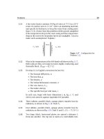
Figure 6.14 The exact and approximate Prandtl number influ-
ence on the ratio of b.l. thicknesses.
Integrating this result with respect to x and taking δ
t
= 0atx = 0, we
get
δ
t
=
3αx
u
∞
3
20
φ −
3
280
φ
3
(6.53)
But δ = 4.64x/
Re
x
in the integral formulation [eqn. (6.31)]. We divide
by this value of δ to be consistent and obtain
δ
t
δ
≡ φ = 0.9638
Pr φ
1 −φ
2
/14
Rearranging this gives
δ
t
δ
=
1
1.025 Pr
1/3
1 −(δ
2
t
/14δ
2
)
1/3
1
1.025 Pr
1/3
(6.54)
The unapproximated result above is shown in Fig. 6.14, along with the
results of Pohlhausen’s precise calculation (see Schlichting [6.3, Chap. 14]).
It turns out that the exact ratio, δ/δ
t
, is represented with great accuracy
304 Laminar and turbulent boundary layers §6.5
by
δ
t
δ
= Pr
−1/3
0.6 Pr 50 (6.55)
So the integral method is accurate within 2.5% in the Prandtl number
range indicated.
Notice that Fig. 6.14 is terminated for Pr less than 0.6. The reason for
doing this is that the lowest Pr for pure gases is 0.67, and the next lower
values of Pr are on the order of 10
−2
for liquid metals. For Pr = 0.67,
δ
t
/δ = 1.143, which violates the assumption that δ
t
δ, but only by a
small margin. For, say, mercury at 100
◦
C, Pr = 0.0162 and δ
t
/δ = 3.952,
which violates the condition by an intolerable margin. We therefore have
a theory that is acceptable for gases and all liquids except the metallic
ones.
The final step in predicting the heat flux is to write Fourier’s law:
q =−k
∂T
∂y
y=0
=−k
T
w
−T
∞
δ
t
∂
T −T
∞
T
w
−T
∞
∂(y/δ
t
)
y/δ
t
=0
(6.56)
Using the dimensionless temperature distribution given by eqn. (6.50),
we get
q =+k
T
w
−T
∞
δ
t
3
2
or
h ≡
q
∆T
=
3k
2δ
t
=
3
2
k
δ
δ
δ
t
(6.57)
and substituting eqns. (6.54) and (6.31) for δ/δ
t
and δ, we obtain
Nu
x
≡
hx
k
=
3
2
Re
x
4.64
1.025 Pr
1/3
= 0.3314 Re
1/2
x
Pr
1/3
Considering the various approximations, this is very close to the result
of the exact calculation, which turns out to be
Nu
x
= 0.332 Re
1/2
x
Pr
1/3
0.6 Pr 50 (6.58)
This expression gives very accurate results under the assumptions on
which it is based: a laminar two-dimensional b.l. on a flat surface, with
T
w
= constant and 0.6 Pr 50.
§6.5 Heat transfer coefficient for laminar, incompressible flow over a flat surface 305
Figure 6.15 A laminar b.l. in a low-Pr liquid. The velocity b.l.
is so thin that u u
∞
in the thermal b.l.
Some other laminar boundary layer heat transfer equations
High Pr. At high Pr, eqn. (6.58) is still close to correct. The exact solution
is
Nu
x
→ 0.339 Re
1/2
x
Pr
1/3
, Pr →∞ (6.59)
Low Pr. Figure 6.15 shows a low-Pr liquid flowing over a flat plate. In
this case δ
t
δ, and for all practical purposes u = u
∞
everywhere within
the thermal b.l. It is as though the no-slip condition [u(y = 0) = 0] and
the influence of viscosity were removed from the problem. Thus, the
dimensional functional equation for h becomes
h = fn
x,k, ρc
p
,u
∞
(6.60)
There are five variables in J/K, m, and s, so there are only two pi-groups.
They are
Nu
x
=
hx
k
and Π
2
≡ Re
x
Pr =
u
∞
x
α
The new group, Π
2
, is called a Péclét number,Pe
x
, where the subscript
identifies the length upon which it is based. It can be interpreted as
follows:
Pe
x
≡
u
∞
x
α
=
ρc
p
u
∞
∆T
k∆T
=
heat capacity rate of fluid in the b.l.
axial heat conductance of the b.l.
(6.61)
306 Laminar and turbulent boundary layers §6.5
So long as Pe
x
is large, the b.l. assumption that ∂
2
T/∂x
2
∂
2
T/∂y
2
will be valid; but for small Pe
x
(i.e., Pe
x
100), it will be violated and a
boundary layer solution cannot be used.
The exact solution of the b.l. equations gives, in this case:
Nu
x
= 0.565 Pe
1/2
x
Pe
x
≥ 100 and
Pr
1
100
or
Re
x
≥ 10
4
(6.62)
General relationship. Churchill and Ozoe [6.5] recommend the follow-
ing empirical correlation for laminar flow on a constant-temperature flat
surface for the entire range of Pr:
Nu
x
=
0.3387 Re
1/2
x
Pr
1/3
1 +
(
0.0468/Pr
)
2/3
1/4
Pe
x
> 100 (6.63)
This relationship proves to be quite accurate, and it approximates eqns.
(6.59) and (6.62), respectively, in the high- and low-Pr limits. The calcu-
lations of an average Nusselt number for the general case is left as an
exercise (Problem 6.10).
Boundary layer with an unheated starting length Figure 6.16 shows
a b.l. with a heated region that starts at a distance x
0
from the leading
edge. The heat transfer in this instance is easily obtained using integral
methods (see Prob. 6.41).
Nu
x
=
0.332 Re
1/2
x
Pr
1/3
1 −
(
x
0
/x
)
3/4
1/3
,x>x
0
(6.64)
Average heat transfer coefficient,
h. The heat transfer coefficient h,is
the ratio of two quantities, q and ∆T , either of which might vary with x.
So far, we have only dealt with the uniform wall temperature problem.
Equations (6.58), (6.59), (6.62), and (6.63), for example, can all be used to
calculate q(x) when (T
w
−T
∞
) ≡ ∆T is a specified constant. In the next
subsection, we discuss the problem of predicting [T (x) −T
∞
] when q is
a specified constant. This is called the uniform wall heat flux problem.
§6.5 Heat transfer coefficient for laminar, incompressible flow over a flat surface 307
Figure 6.16 A b.l. with an unheated region at the leading edge.
The term h is used to designate either q/∆T in the uniform wall tem-
perature problem or q/
∆T in the uniform wall heat flux problem. Thus,
uniform wall temp.:
h ≡
q
∆T
=
1
∆T
1
L
L
0
qdx
=
1
L
L
0
h(x) dx
(6.65)
uniform heat flux:
h ≡
q
∆T
=
q
1
L
L
0
∆T(x)dx
(6.66)
The Nusselt number based on
h and a characteristic length, L, is desig-
nated
Nu
L
. This is not to be construed as an average of Nu
x
, which would
be meaningless in either of these cases.
Thus, for a flat surface (with x
0
= 0), we use eqn. (6.58) in eqn. (6.65)
to get
h =
1
L
L
0
h(x) dx
k
x
Nu
x
=
0.332 k Pr
1/3
L
u
∞
ν
L
0
√
xdx
x
= 0.664 Re
1/2
L
Pr
1/3
k
L
(6.67)
Thus,
h = 2h(x = L) in a laminar flow, and
Nu
L
=
hL
k
= 0.664 Re
1/2
L
Pr
1/3
(6.68)
Likewise for liquid metal flows:
Nu
L
= 1.13 Pe
1/2
L
(6.69)
308 Laminar and turbulent boundary layers §6.5
Some final observations. The preceding results are restricted to the
two-dimensional, incompressible, laminar b.l. on a flat isothermal wall at
velocities that are not too high. These conditions are usually met if:
• Re
x
or Re
L
is not above the turbulent transition value, which is
typically a few hundred thousand.
• The Mach number of the flow, Ma ≡ u
∞
/(sound speed), is less than
about 0.3. (Even gaseous flows behave incompressibly at velocities
well below sonic.) A related condition is:
• The Eckert number,Ec≡ u
2
∞
/c
p
(T
w
−T
∞
), is substantially less than
unity. (This means that heating by viscous dissipation—which we
have neglected—does not play any role in the problem. This as-
sumption was included implicitly when we treated J as an indepen-
dent unit in the dimensional analysis of this problem.)
It is worthwhile to notice how h and Nu depend on their independent
variables:
h or
h ∝
1
√
x
or
1
√
L
,
√
u
∞
,ν
−1/6
,(ρc
p
)
1/3
,k
2/3
Nu
x
or Nu
L
∝
x or L,
√
u
∞
,ν
−1/6
,(ρc
p
)
1/3
,k
−1/3
(6.70)
Thus, h →∞and Nu
x
vanishes at the leading edge, x = 0. Of course,
an infinite value of h, like infinite shear stress, will not really occur at
the leading edge because the b.l. description will actually break down in
a small neighborhood of x = 0.
In all of the preceding considerations, the fluid properties have been
assumed constant. Actually, k, ρc
p
, and especially µ might all vary no-
ticeably with T within the b.l. It turns out that if properties are all eval-
uated at the average temperature of the b.l. or film temperature T
f
=
(T
w
+T
∞
)/2, the results will normally be quite accurate. It is also worth
noting that, although properties are given only at one pressure in Ap-
pendix A; µ, k, and c
p
change very little with pressure, especially in liq-
uids.
Example 6.5
Air at 20
◦
C and moving at 15 m/s is warmed by an isothermal steam-
heated plate at 110
◦
C, ½ m in length and½minwidth. Find the
average heat transfer coefficient and the total heat transferred. What
are h, δ
t
, and δ at the trailing edge?
§6.5 Heat transfer coefficient for laminar, incompressible flow over a flat surface 309
Solution. We evaluate properties at T
f
= (110+20)/2 = 65
◦
C. Then
Pr = 0.707 and Re
L
=
u
∞
L
ν
=
15(0.5)
0.0000194
= 386, 600
so the flow ought to be laminar up to the trailing edge. The Nusselt
number is then
Nu
L
= 0.664 Re
1/2
L
Pr
1/3
= 367.8
and
h = 367.8
k
L
=
367.8(0.02885)
0.5
= 21.2 W/m
2
K
The value is quite low because of the low conductivity of air. The total
heat flux is then
Q =
hA ∆T = 21.2(0.5)
2
(110 −20) = 477 W
By comparing eqns. (6.58) and (6.68), we see that h(x = L) = ½
h,so
h(trailing edge) =
1
2
(21.2) = 10.6 W/m
2
K
And finally,
δ(x = L) = 4.92L
Re
L
=
4.92(0.5)
386, 600
= 0.00396 m
= 3.96 mm
and
δ
t
=
δ
3
√
Pr
=
3.96
3
√
0.707
= 4.44 mm
The problem of uniform wall heat flux
When the heat flux at the heater wall, q
w
, is specified instead of the
temperature, it is T
w
that we need to know. We leave the problem of
finding Nu
x
for q
w
= constant as an exercise (Problem 6.11). The exact
result is
Nu
x
= 0.453 Re
1/2
x
Pr
1/3
for Pr 0.6 (6.71)
310 Laminar and turbulent boundary layers §6.5
where Nu
x
= hx/k = q
w
x/k(T
w
− T
∞
). The integral method gives the
same result with a slightly lower constant (0.417).
We must be very careful in discussing average results in the constant
heat flux case. The problem now might be that of finding an average
temperature difference (cf. (6.66)):
T
w
−T
∞
=
1
L
L
0
(T
w
−T
∞
)dx =
1
L
L
0
q
w
x
k(0.453
u
∞
/ν Pr
1/3
)
dx
√
x
or
T
w
−T
∞
=
q
w
L/k
0.6795 Re
1/2
L
Pr
1/3
(6.72)
which can be put into the form
Nu
L
= 0.6795 Re
1/2
L
Pr
1/3
(although the
Nusselt number yields an awkward nondimensionalization for
T
w
−T
∞
).
Churchill and Ozoe [6.5] have pointed out that their eqn. (6.63) will de-
scribe (T
w
− T
∞
) with high accuracy over the full range of Pr if the con-
stants are changed as follows:
Nu
x
=
0.4637 Re
1/2
x
Pr
1/3
1 +
(
0.02052/Pr
)
2/3
1/4
Pe
x
> 100 (6.73)
Example 6.6
Air at 15
◦
C flows at 1.8m/s over a 0.6 m-long heating panel. The
panel is intended to supply 420 W/m
2
to the air, but the surface can
sustain only about 105
◦
C without being damaged. Is it safe? What is
the average temperature of the plate?
Solution. In accordance with eqn. (6.71),
∆T
max
= ∆T
x=L
=
qL
k Nu
x=L
=
qL/k
0.453 Re
1/2
x
Pr
1/3
or if we evaluate properties at (85 +15)/2 = 50
◦
C, for the moment,
∆T
max
=
420(0.6)/0.0278
0.453
0.6(1.8)/1.794 ×10
−5
1/2
(0.709)
1/3
= 91.5
◦
C
This will give T
w
max
= 15 + 91.5 = 106.5
◦
C. This is very close to
105
◦
C. If 105
◦
C is at all conservative, q = 420 W/m
2
should be safe—
particularly since it only occurs over a very small distance at the end
of the plate.
§6.6 The Reynolds analogy 311
From eqn. (6.72) we find that
∆T =
0.453
0.6795
∆T
max
= 61.0
◦
C
so
T
w
= 15 + 61.0 = 76.0
◦
C
6.6 The Reynolds analogy
The analogy between heat and momentum transfer can now be general-
ized to provide a very useful result. We begin by recalling eqn. (6.25),
which is restricted to a flat surface with no pressure gradient:
d
dx
δ
1
0
u
u
∞
u
u
∞
−1
d
y
δ
=−
C
f
2
(6.25)
and by rewriting eqns. (6.47) and (6.51), we obtain for the constant wall
temperature case:
d
dx
φδ
1
0
u
u
∞
T −T
∞
T
w
−T
∞
d
y
δ
t
=
q
w
ρc
p
u
∞
(T
w
−T
∞
)
(6.74)
But the similarity of temperature and flow boundary layers to one another
[see, e.g., eqns. (6.29) and (6.50)], suggests the following approximation,
which becomes exact only when Pr = 1:
T −T
∞
T
w
−T
∞
δ =
1 −
u
u
∞
δ
t
Substituting this result in eqn. (6.74) and comparing it to eqn. (6.25), we
get
−
d
dx
δ
1
0
u
u
∞
u
u
∞
−1
d
y
δ
=−
C
f
2
=−
q
w
ρc
p
u
∞
(T
w
−T
∞
)φ
2
(6.75)
Finally, we substitute eqn. (6.55) to eliminate φ from eqn. (6.75). The
result is one instance of the Reynolds-Colburn analogy:
8
h
ρc
p
u
∞
Pr
2/3
=
C
f
2
(6.76)
8
Reynolds [6.6] developed the analogy in 1874. Colburn made important use of it in
this century. The form given is for flat plates with 0.6 ≤ Pr ≤ 50. The Prandtl number
factor is usually a little different for other flows or other ranges of Pr.
312 Laminar and turbulent boundary layers §6.6
For use in Reynolds’ analogy, C
f
must be a pure skin friction coefficient.
The profile drag that results from the variation of pressure around the
body is unrelated to heat transfer. The analogy does not apply when
profile drag is included in C
f
.
The dimensionless group h/ρc
p
u
∞
is called the Stanton number.It
is defined as follows:
St, Stanton number ≡
h
ρc
p
u
∞
=
Nu
x
Re
x
Pr
The physical significance of the Stanton number is
St =
h∆T
ρc
p
u
∞
∆T
=
actual heat flux to the fluid
heat flux capacity of the fluid flow
(6.77)
The group St Pr
2/3
was dealt with by the chemical engineer Colburn, who
gave it a special symbol:
j ≡ Colburn j-factor = St Pr
2/3
=
Nu
x
Re
x
Pr
1/3
(6.78)
Example 6.7
Does the equation for the Nusselt number on an isothermal flat sur-
face in laminar flow satisfy the Reynolds analogy?
Solution. If we rewrite eqn. (6.58), we obtain
Nu
x
Re
x
Pr
1/3
= St Pr
2/3
=
0.332
Re
x
(6.79)
But comparison with eqn. (6.33) reveals that the left-hand side of
eqn. (6.79) is precisely C
f
/2, so the analogy is satisfied perfectly. Like-
wise, from eqns. (6.68) and (6.34), we get
Nu
L
Re
L
Pr
1/3
≡ St Pr
2/3
=
0.664
Re
L
=
C
f
2
(6.80)
The Reynolds-Colburn analogy can be used directly to infer heat trans-
fer data from measurements of the shear stress, or vice versa. It can also
be extended to turbulent flow, which is much harder to predict analyti-
cally. We shall undertake that problem in Sect. 6.8.
§6.7 Turbulent boundary layers 313
Example 6.8
How much drag force does the air flow in Example 6.5 exert on the
heat transfer surface?
Solution. From eqn. (6.80) in Example 6.7, we obtain
C
f
=
2
Nu
L
Re
L
Pr
1/3
From Example 6.5 we obtain Nu
L
,Re
L
, and Pr
1/3
:
C
f
=
2(367.8)
(386, 600)(0.707)
1/3
= 0.002135
so
τ
yx
= (0.002135)
1
2
ρu
2
∞
=
(0.002135)(1.05)(15)
2
2
= 0.2522 kg/m·s
2
and the force is
τ
yx
A = 0.2522(0.5)
2
= 0.06305 kg·m/s
2
= 0.06305 N
= 0.23 oz
6.7 Turbulent boundary layers
Turbulence
Big whirls have little whirls,
That feed on their velocity.
Little whirls have littler whirls,
And so on, to viscosity.
This bit of doggerel by the English fluid mechanic, L. F. Richardson, tells
us a great deal about the nature of turbulence. Turbulence in a fluid can
be viewed as a spectrum of coexisting vortices in which kinetic energy
from the larger ones is dissipated to successively smaller ones until the
very smallest of these vortices (or “whirls”) are damped out by viscous
shear stresses.
The next time the weatherman shows a satellite photograph of North
America on the 10:00 p.m. news, notice the cloud patterns. There will be