Báo cáo toán học: "Tensorial Square of the Hyperoctahedral Group Coinvariant Space" ppt

Tensorial Square of the Hyperoctahedral Group
Coinvariant Space
Fran¸cois Bergeron
∗
D´epartement de Math´ematiques
Universit´eduQu´ebec `aMontr´eal
Montr´eal, Qu´ebec, H3C 3P8, CANADA

Riccardo Biagioli
Institut Camille Jordan
Universit´e Claude Bernard Lyon 1
69622 Villeurbanne, FRANCE

Submitted: Jul 21, 2005; Accepted: Mar 28, 2006; Published: Apr 11, 2006
Mathematics Subject Classifications: 05E05, 05E15
Abstract
The purpose of this paper is to give an explicit description of the trivial and alter-
nating components of the irreducible representation decomposition of the bigraded
module obtained as the tensor square of the coinvariant space for hyperoctahedral
groups.
1 Introduction.
The group B
n
×B
n
,withB
n
the group of “signed” permutations, acts in the usual natural
way as a “reflection group” on the polynomial ring in two sets of variables
Q[x, y]=Q[x
1

, ,x
n
,y
1
, ,y
n
], (β,γ)(x
i
,y
j
)=(±x
σ(i)
, ±y
τ(j)
),
where ± denotes some appropriate sign, and σ and τ are the unsigned permutations
corresponding respectively to β and γ. Let us denote I
B×B
the ideal generated by constant
term free invariant polynomials for this action. We then consider the “coinvariant space”
C = Q[x, y]/I
B×B
for the group B
n
× B
n
. It is well known [12, 13, 17, 18] that C is
∗
F. Bergeron is supported in part by NSERC-Canada and FQRNT-Qu´ebec
the electronic journal of combinatorics 13 (2006), #R38 1

isomorphic to the regular representation of B
n
× B
n
, since it acts here as a reflection
group.
The purpose of this paper is to study the isotypic components of C with respect to the
action of B
n
rather then that of B
n
× B
n
. This is to say that we are restricting the action
to B
n
, here considered as a “diagonal” subgroup of B
n
× B
n
. It is worth underlying that
this is not a reflection groups action, and so we are truly in front of a new situation with
respect to the classical results alluded to above. Part of the results we obtain consists
in giving explicit descriptions of the trivial and alternating components of the space C.
We will see that in doing so, we are lead to introduce two new classes of combinatorial
objects respectfully called compact e-diagrams and compact o-diagrams. Wegiveanice
bijection between natural n-element subsets of N × N indexing “diagonal B
n
-invariants”,
and triples (D

β
,λ,µ), where λ and µ are partitions with at most n parts, and D
β
is
acompacte-diagram. A similar result will be obtained for “diagonal B
n
-alternants”,
involving compact o-diagram in this case. As we will also see, both families of compact
diagrams are naturally indexed by signed permutations.
One of the many reasons to study the coinvariant space C is that it strictly contains
the space of “diagonal coinvariants” of B
n
in a very natural way. This will be further
discussed in Section 3. This space of diagonal coinvariants was recently characterized by
Gordon [9] in his solution of conjectures of Haiman [11], (see also, [4], [10], and [14]).
Moreover, the space C contains some of the spaces that appear in the work of Allen [2],
namely those that are generated by B
n
-alternants that are contained in C.Usingour
Theorem 15.2 one can readily check that the join of these spaces is strictly contained as
a subspace of C.
The paper is organized as follows. We start with a general survey of classical re-
sults regarding coinvariant spaces of finite reflection groups, followed with implications
regarding the tensor square of these same spaces. We then specialize our discussion to
hyperoctahedral groups, recalling in the process the main aspects of their representation
theory relating to the B
n
-Frobenius transform of characters. Many of these results have
already appeared in scattered publications but are hard to find in a unified presentation.
We then finally proceed to introduce our combinatorial tools and derive our main results.

2 Reflection group action on the polynomial ring
For any finite reflection group W , on a finite dimensional vector space V over Q,there
corresponds a natural action of W on the polynomial ring Q[V ]. In particular, if x =
x
1
, ,x
n
is a basis of V then Q[V ] can be identified with the ring Q[x] of polynomials
in the variables x
1
, ,x
n
. As usual, we denote
w · p(x)=p(w · x),
the action in question. It is clear that this action of W is degree preserving, thus making
natural the following considerations. Let us denote π
d
(p(x)) the degree d homogeneous
the electronic journal of combinatorics 13 (2006), #R38 2
component of a polynomial p(x). The ring Q := Q[x] is graded by degree, hence
Q 

d≥0
Q
d
,
where Q
d
:= π
d

(Q)isthedegree d homogeneous component of Q. Recall that a subspace
S is said to be homogeneous if π
d
(S) ⊆ S for all d. Whenever this is the case, we clearly
have S =

d≥0
S
d
,withS
d
:= S ∩ Q
d
, and thus it makes sense to consider the Hilbert
series of S:
H
q
(S):=

m≥0
dim(S
d
) q
d
.
The motivation, behind the introduction of this formal power series in q,isthatitcon-
denses in a efficient and compact form the information for the dimensions of each of the
S
d
’s. To illustrate, it is not hard to show that the Hilbert series of Q is simply

H
q
(Q)=
1
(1 − q)
n
, (2.1)
which is equivalent to the infinite list of statements
dim(Q
d
)=

n + d − 1
d

,
one for each value of d.
We will be particularly interested in invariant subspaces S of Q, namely those for
which w · S ⊆ S, for all w in W . Clearly whenever S is homogeneous, on top of being
invariant, then each of these homogeneous component, S
d
,isalsoaW -invariant subspace.
One important example of homogeneous invariant subspace, denoted Q
W
,isthesetof
invariant polynomials. These are the polynomials p(x) such that
w · p(x)=p(x).
Here, not only the subspace Q
W
is invariant, but all of its elements are. It is well know

that Q
W
is in fact a subring of Q, for which one can find generator sets of n homoge-
neous algebraically independent elements, say f
1
, ,f
n
, whose respective degrees will be
denoted d
1
, ,d
n
. Although the f
i
’s are not uniquely characterized, the d
i
’s are basic
numerical invariants of the group, called the degrees of W .Anyn-set {f
1
, ,f
n
} of
invariants with these properties is called a set of basic invariants for W . It follows that
the Hilbert series of Q
W
takes the form:
H
q
(Q
W

)=
n

i=1
1
1 − q
d
i
. (2.2)
Now, let I
W
be the ideal of Q generated by constant term free elements of Q
W
.The
coinvariant space of W is defined to be
Q
W
:= Q/I
W
. (2.3)
the electronic journal of combinatorics 13 (2006), #R38 3
Observe that, since I
W
is an homogeneous subspace of Q, it follows that the ring Q
W
is
naturally graded by degree. Moreover, I
W
being W -invariant, the group W acts naturally
on Q

W
. In fact, it can be shown that Q
W
is actually isomorphic to the left regular
representation of W (For more on this see [13] or [17]). It follows that the dimension of
Q
W
is exactly the order of the group W . We can get a finer description of this fact using
a theorem of Chevalley (see [12, Section 3.5]) that can be stated as follows. There exists
a natural isomorphism of QW -module
1
:
Q  Q
W
⊗ Q
W
. (2.4)
We will use strongly this decomposition in the rest of the paper. One immediate conse-
quence, in view of (2.1) and (2.2), is that
H
q
(Q
W
)=
n

i=1
1 − q
d
i

1 − q
(2.5)
=(1+···+ q
d
1
−1
) ···(1 + ···+ q
d
n
−1
).
We now introduce another important QW -module for our discussion. To describe it, let
us first introduce a W -invariant scalar product on Q,namely
p, q := p(∂x)q(x)|
x=0
.
Here p(∂x) stands for the linear operator obtained by replacing each variable x
i
,inthe
polynomial p(x), by the partial derivative ∂x
i
with respect to x
i
. We have denoted above
by x = 0 the simultaneous substitutions x
i
= 0, one for each i. With this in mind, we
define the space of W-harmonic polynomials:
H
W

:= I
⊥
W
(2.6)
where, as usual, ⊥ stands for orthogonal complement with respect to the underlying scalar
product. Equivalently, since I
W
is can be described as the ideal generated (as above) by
abasicset{f
1
, ,f
n
} of invariants, then a polynomial p(x)isinH
W
if and only if
f
k
(∂x)p(x)=0, for all k ≥ 0.
It can be shown that the spaces H
W
and Q
W
are actually isomorphic as graded QW-
modules [18]. On the other hand, it is easy to observe that H
W
is closed under partial
derivatives. These observations, together with a further remark about characterizations of
reflection groups contained in Chevalley’s Theorem, make possible an explicit description
of H
W

in term of the Jacobian determinant:
∆
W
(x):=
1
|W |
det
∂f
i
∂x
j
, (2.7)
1
Here, as usual, QW stands for the group algebra of W ,andthetermmodule underlines that we are
extending the action of W to its group algebra.
the electronic journal of combinatorics 13 (2006), #R38 4
where the f
i
’s form a set of basic W -invariants. This polynomial is also simply denoted
∆(x), when the underlying group is clear. One can show that this polynomial is well
defined (up to a scalar multiple) in that it does not depend on the actual choice of the
f
i
’s (see [12, Section 3.13]). It can also be shown that ∆
W
is the unique (up to scalar
multiple) W -harmonic polynomial of maximal degree, and we have
H
W
= L

∂
[∆
W
(x)], (2.8)
where L
∂
stands as short hand for “linear span of all partial derivatives of”. Another
important property of ∆ = ∆
W
is that it allows an explicit characterization of all W -
alternating polynomials. Recall that, p(x)issaidtobeW -alternating if and only if
w · p(x)=det(w) p(x),
where, to make sense out of det(w), one interprets w as linear transformation. The
pertinent statement is that p(x) is alternating if and only if it can be written as
p(x)=f(x)∆(x),
with f(x)inQ
W
. In other words, ∆ is the minimal W -alternating polynomial. Thus, in
view of (2.2) and (2.7), the Hilbert series of the homogeneous invariant subspace Q
±
,of
W -alternating polynomials, is simply
H
q
(Q
±
)=
n

i=1

q
d
i
−1
1 − q
d
i
. (2.9)
The point of all this is that we can reformulate the decomposition given in (2.4) as
Q  Q
W
⊗H
W
, (2.10)
with both Q
W
and H
W
W -submodules of Q. In other words, there is a unique decompo-
sition of any polynomial p(x) of the form
p(x)=

w∈W
f
w
(x) b
w
(x),
for any given basis {b
w

(x) | w ∈ W } of H
W
,withthef
w
(x)’s invariant polynomials.
Recall here that H
W
has dimension equal to |W |. As we will see in particular instances,
there are natural choices for such a basis.
3 Diagonally invariant and alternating polynomials
We now extend our discussion to the ring
R = Q[x, y]:=Q[x
1
, ,x
n
,y
1
, ,y
n
],
the electronic journal of combinatorics 13 (2006), #R38 5
of polynomials in two sets of n variables, on which we want to study the diagonal action
of W , namely such that:
w · p(x, y)=p(w · x,w· y), (3.1)
for w ∈ W .Inthiscase,W does not act as a reflection group on the vector space V
spanned by the x
i
’s and y
j
’s, so that we are truly in front of a new situation, as we will

see in more details below. By comparison, the results of Section 2 would still apply to R
if we would rather consider the action of W × W , for which
(w, τ) · p(x, y)=p(w · x,τ · y), (3.2)
when (w, τ) ∈ W × W ,andp(x, y) ∈ R. Indeed, this does correspond to an action of
W × W as a reflection group on V. Each of these two contexts give rise to a notion of
invariant polynomials in the same space R. Notation wise, we naturally distinguish these
two notions as follows. On one hand we have the subring R
W
of diagonally invariant
polynomials, namely those for which
p(w · x,w· y)=p(x, y); (3.3)
and, on the other hand, we get the subring R
W ×W
, of invariants polynomials of the tensor
action (3.2), as a special case of the results described in Section 2. Observe that
R
W ×W
 Q[x]
W
⊗ Q[y]
W
. (3.4)
In view of this observation, we will called R
W ×W
the tensor invariant algebra.Itiseasy
to see that R
W ×W
is a subring of R
W
.

The ring R is naturally “bigraded” with respect to “bidegree”. To make sense out of
this, let us recall the usual vectorial notation for monomials:
x
a
y
b
:= x
a
1
1
···x
a
n
n
y
b
1
1
···y
b
n
n
,
with a =(a
1
, ,a
n
)andb =(b
1
, ,b

n
)bothinN
n
. Then, the bidegree of x
a
y
b
is
simply (|a|, |b|), where |a| stands for the sum of the components of a, and likewise for b.
If we now introduce the linear operator π
k,j
such that
π
k,j
(x
a
y
b
):=

x
a
y
b
if |a| = k and |b| = j,
0 otherwise,
then a polynomial p(x, y)issaidtobebihomogeneous of bidegree (k, j) if and only if
π
k,j
(p(x, y)) = p(x, y).

The notion of bigrading is then obvious. For instance, we have the bigraded decomposition:
R =

k,j
R
k,j
,
the electronic journal of combinatorics 13 (2006), #R38 6
with R
k,j
:= π
k,j
(R). Naturally, a subspace S of R is said to be bihomogeneous if π
k,j
(S) ⊆
S for all k and j, and it is just as natural to consider the bigraded Hilbert series:
H
q,t
(S):=

k,j
dim(S
k,j
)q
k
t
j
,
with S
k,j

:= S ∩ R
k,j
. Since it is clear that
R  Q[x] ⊗ Q[y],
from (2.1) we easily get
H
q,t
(R)=
1
(1 − q)
n
1
(1 − t)
n
. (3.5)
Furthermore, in view of (3.4) and (2.2), the bigraded Hilbert series of R
W ×W
is simply
H
q,t
(R
W ×W
)=
n

i=1
1
(1 − q
d
i

)(1 − t
d
i
)
. (3.6)
Let R
W ×W
and H
W ×W
the spaces of coinvariants and harmonics of W × W, defined in
(2.3) and (2.6), respectively. From (3.5) and (3.6), we conclude that
H
q,t
(R
W ×W
)=H
q,t
(H
W ×W
)
=
n

i=1
1 − q
d
i
1 − q
n


i=1
1 − t
d
i
1 − t
. (3.7)
In fact, we have (W × W )-module isomorphisms of bigraded spaces
CQ
W
⊗ Q
W
(3.8)
HH
W
⊗H
W
. (3.9)
Here, and from now on, we simply denote C the space of coinvariants of W × W ,andH
the space of harmonics of W × W . Recalling our previous general discussion, the spaces
C and H are isomorphic as bigraded W -modules. Summing up, and considering W as a
diagonal subgroup of W × W (i.e.: w → (w, w)) we get an isomorphism of W -module
R  Q[x]
W
⊗ Q[y]
W
⊗H (3.10)
from which we deduce, in particular, that
R
W
 Q[x]

W
⊗ Q[y]
W
⊗H
W
, (3.11)
where
H
W
:= R
W
∩H.
Similarly, for the W -module of diagonally alternating polynomials
R
±
:= {p(x, y) ∈ R | p(w · x,w· y)=det(w) p(x, y)}, (3.12)
the electronic journal of combinatorics 13 (2006), #R38 7
we have the decomposition:
R
±
 Q[x]
W
⊗ Q[y]
W
⊗H
±
, (3.13)
where
H
±

:= R
±
∩H.
Thus the two spaces H
W
and H
±
, respectively of diagonally symmetric and diagonally
alternating harmonic polynomials, play a special role in the understanding of of R
W
and
R
±
. As we will see below, they are also very interesting on their own. Clearly, H
W
C
W
and H
±
C
±
. Nice combinatorial descriptions of these two last spaces will be given in
thecaseofWeylgroupsoftypeB.
As briefly announced in the introduction, the coinvariant space C strictly contains the
space of diagonal coinvariants D
B
such as characterized by Gordon. More precisely (see
[9] for details) this last space is a subspace of the quotient R/J
B
,whereJ

B
is the ideal
generated by all constant term free B
n
-diagonally invariant polynomial defined in (3.3).
SincewehavealreadyseenthatJ
B
⊃I
B×B
, we concluded that D
B
⊂C,sincethetwo
relevant ideals are clearly very different. Along this line it is worth recalling that D
B
has
dimension (2n +1)
n
, whereas we already know that the dimension of C is the much larger
value (2
n
n!)
2
. Many interesting questions regarding D
B
are still unsolved. We hope that
our investigations will shed some light on this fascinating topic through the study of of a
nice overspace.
4 The Hyperoctahedral group B
n
The hyperoctahedral group B

n
is the group of signed permutations of the set [n]:=
{1, 2, ,n}. More precisely, it is obtained as the wreath product, Z
2
 S
n
,ofthe“sign
change” group Z
2
and the symmetric group S
n
. In one line notation, elements of B
n
can
be written as
β = β(1)β(2) ···β(n),
with each β(i) an integer whose absolute value lies in [n]. Moreover, if we replace in β
each these β(i)’s by their absolute value, we get a permutation. We often denote the
negative entries with an overline, thus
2 1 543∈ B
5
.
The action of β in B
n
on polynomials is entirely characterized by its effect on variables:
β · x
i
= ±x
σ(i)
,

with the sign equal to the sign of β(i), and σ(i) equal to its absolute value. The B
n
-
invariant polynomials are thus simply the usual symmetric polynomials in the square of
the variables. We will write
f(x
2
):=f(x
2
1
,x
2
2
, ,x
2
n
).
Hence a set of basic invariant for Q
B
n
is given by the power sum symmetric polynomials:
p
j
(x
2
)=

1≤k≤n
x
2j

k
,
the electronic journal of combinatorics 13 (2006), #R38 8
with j going from 1 to n.Thus2, 4, ,2n are the degrees of B
n
and from (2.2) we get
H
q
(Q
B
n
)=
n

i=1
1
(1 − q
2i
)
. (4.1)
It also follows that the Jacobian determinant (2.7) is
∆(x)=
1
2
n
n!
det






11 1
2x
1
2x
2
2x
n
.
.
.
.
.
.
.
.
.
.
.
.
2nx
2n−1
1
2nx
2n−1
2
2nx
2n−1
n






which factors out simply as
∆(x)=x
1
···x
n

1≤i<j≤n
(x
2
i
− x
2
j
). (4.2)
Now, an easy application of Buchberger’s criteria (see e.g., [6]) shows that the set
{h
k
(x
2
k
, ,x
2
n
) | 1 ≤ k ≤ n} (4.3)
is a Gr¨obner basis for the ideal I = I

B
n
. Here, we are using the lexicographic monomial
order (with the variables ordered as x
1
>x
2
> >x
n
), and h
k
denotes the k
th
complete
homogeneous symmetric polynomial. It follows from the corresponding theory that a linear
basis for the coinvariant space Q
B
n
= Q/I is given by the set
{x

+ I| =(
1
, ,
n
), with 0 ≤ 
i
< 2i}. (4.4)
These monomials are exactly those that are not divisible by any of the leading terms
x

2
1
, ,x
2k
k
, ,x
2n
n
of the polynomials in the Gr¨obner basis (4.3). The linear basis (4.4) is sometimes called the
Artin basis of the coinvariant space. If we systematically order the terms of polynomials
in decreasing lexicographic order, it is then easy to deduce, from (2.8) and (4.4), that the
set
{∂x

∆(x) |  =(
1
, ,
n
), 0 ≤ 
i
< 2i}.
is a basis of the module of B
n
-harmonic polynomials. This makes it explicit that 2
n
n!is
the dimension of both Q
B
n
and H

B
n
. We will often go back and forth between Q
B
n
and
H
B
n
, using the fact that they are isomorphic as graded representations of B
n
.
Another basis of the space of coinvariants, called the descent basis, will be useful for
our purpose. Let us first introduce some “statistics” on B
n
that also have an important
role in our presentation. We start by fixing the following linear order on Z:
¯
1 ≺
¯
2 ≺···≺ ¯n ≺···≺0 ≺ 1 ≺ 2 ≺···≺n ≺··· .
the electronic journal of combinatorics 13 (2006), #R38 9
Then, following [1], we define the flag-major index of β ∈ B
n
by
fmaj(β):=2maj(β)+neg(β), (4.5)
where neg(β) is just the number of the negative entries in β,andmaj(β) is the usual
major index of an integer sequence, i.e.,
maj(β)=


i∈Des(β)
i.
Here, Des(β) stands for the descent set of β,namely
Des(β):={i ∈ [n − 1] | β
i
 β
i+1
}.
For example, with β =
¯
2
¯
1
¯
5 4 3, we get Des(β)={1, 4},maj(β)=5,neg(β) = 3, and
fmaj(β) = 15. It will be handy to localize these three statistics setting, for i ∈ [n]:
f
i
(β):=2d
i
(β)+ε
i
(β), with (4.6)
ε
i
(β):=

1ifβ(i) < 0, and
0 otherwise,
(4.7)

d
i
(β):=#{j ∈ Des(β) | j ≥ i}. (4.8)
As is shown in [3], the set {x
β
+ I|β ∈ B
n
}, with
x
β
:=
n

i=1
x
f
i
(β)
σ(i)
,
is another linear basis of the coinvariant space Q
B
n
,ifσ(i) denotes the absolute value of
β(i). Note that each monomial x
β
has precisely degree fmaj(β) so that, in view of (2.5)
we get

β∈B

n
q
fmaj(β)
=
n

j=1
1 − q
2j
1 − q
.
5 Plethystic substitution
To go on with our discussion, it will be particularly efficient to use the notion of “plethystic
substitution”. Let z = z
1
,z
2
,z
3
, and
¯
z =¯z
1
, ¯z
2
, ¯z
3
, be two infinite sets of “formal”
variables, and denote Λ(z) (resp. Λ(
¯

z)) the ring of symmetric functions
2
in these variables
z (resp.
¯
z). It is well known that any classical linear basis of Λ(z) is naturally indexed
by partitions. We usually denote  = (λ) the number of parts of λ  n (λ “a partition
of” n). In accordance with the notation of [15], we further denote
p
λ
(z):=p
λ
1
(z)p
λ
2
(z) ···p
λ

(z),
2
Here, the term “function” is used to emphasize that we are dealing with infinitely many variables.
the electronic journal of combinatorics 13 (2006), #R38 10
the power sum symmetric function indexed by the partition λ = λ
1
λ
2
···λ

. The homo-

geneous degree n complete and elementary symmetric functions are respectively denoted
by h
n
(z)ande
n
(z). Recall that we have

n≥0
h
n
(z)t
n
=exp


k≥1
p
k
(z)t
k
/k

, and

n≥0
e
n
(z)t
n
=exp



k≥1
(−1)
k−1
p
k
(z)t
k
/k

.
Our intent here is to use symmetric functions expressions, obtained by “plethystic sub-
stitution”, to encode characters. A plethystic substitution u[w], of an expression w into
a symmetric function u, is defined as follows. The first ingredient used to “compute” the
resulting expression, is the fact that such a substitution is both additive and multiplica-
tive:
(u + v)[w]=u[w]+v[w]
(uv)[w]=u[w] v[w].
Moreover, a plethystic substitution into a power sum p
k
is defined to result in replacing
all variables in w by their k
th
power. In particular, this makes such a substitution linear
in the argument p
k
[w
1
+ w

2
]=p
k
[w
1
]+p
k
[w
2
]. Summing up, we get
u[w]:=

µ
a
µ
(µ)

i=1
p
µ
i
[w]
whenever the expansion of u in power sum is u(z):=

µ
a
µ
p
µ
(z).

A further useful convention, in this context, is to denote sets of variables z
1
,z
2
,z
3
, ,
as (formal) sums z = z
1
+ z
2
+ z
3
+ This has the nice feature that the result of the
plethystic substitution of a “set” of variables into a power sum p
k
:
p
k
[z]=p
k
[z
1
+ z
2
+ z
3
+ ]
= z
k

1
+ z
k
2
+ z
k
3
+
is exactly the corresponding power sum in this set of variables. As an illustration of the
many useful formulas one can get using this approach, we have
h
n
[w
1
+ w
2
]=
n

k=0
h
k
[w
1
]h
n−k
[w
2
] (5.1)
as well as

h
n
[w
1
w
2
]=

λn
s
λ
[w
1
]s
λ
[w
2
], (5.2)
where the s
λ
’s are the classical Schur functions. Recall that
s
λ
(z)=

µ
χ
λ
µ
p

µ
(z)
z
µ
, (5.3)
the electronic journal of combinatorics 13 (2006), #R38 11
where
χ
λ
µ
is the value at µ of the irreducible character of S
n
associated to a partition λ,
and we have set
z
µ
:= 1
k
1
k
1
!2
k
2
k
2
! ···n
k
n
k

n
! (5.4)
whenever µ has k
i
parts of size i. It is well known that conjugacy classes of S
n
are
naturally indexed by partitions, hence (5.3) is an encoding of the character table of S
n
.
Moreover, the s
λ
’s have a natural role in computations regarding characters of S
n
, through
the Frobenius characteristic transformation. Recall that this is the symmetric function
associated to a representation V of S
n
, in the following manner
F(V):=
1
n!

σ∈S
n
χ
V
(σ)p
µ(σ)
, (5.5)

where µ(σ) is the partition giving the cycle index structure of σ. It is interesting to illus-
trate this with the regular representation of S
n
, for which the Frobenius (characteristic)
is
p
1
(z)
n
=

λn
f
λ
s
λ
(z). (5.6)
The left hand side corresponds to the direct computation of (5.5), and the right hand
side describe the usual decomposition of the regular representation in terms of irreducible
representations. Here is exemplified the fact that the s
λ
’s correspond to irreducible repre-
sentations of S
n
, through the Frobenius characteristic. A well known fact of representation
theory says that the coefficients f
λ
, in (5.6), are both the dimension of irreducible repre-
sentations of S
n

, and the multiplicities of these in the regular representation. As is also
very well known, these values are given by the hook length formula.
Formulas (5.1) and (5.2) are special cases of the more general formulas:
s
λ
[w
1
+ w
2
]=

ν⊆λ
s
ν
[w
1
]s
λ/ν
[w
2
]
s
λ
[w
1
− w
2
]=

ν⊆λ

(−1)
|λ/ν|
s
ν
[w
1
]s
λ

/ν

[w
2
]
s
λ/µ
[−w]=(−1)
|λ/µ|
s
λ

/µ

[w].
As a particular case of this last formula, we get
h
n
[−w]=(−1)
n
e

n
[w],
since s
(n)
= h
n
and s
1
n
= e
n
. Moreover, we have
h
n
[w]=

µn
1
z
µ
p
µ
[w]. (5.7)
It will be useful also to introduce
Ω[w]:=

n≥0
h
n
[w].

Note that
Ω[w
1
+ w
2
]=Ω[w
1
]Ω[w
2
]. (5.8)
the electronic journal of combinatorics 13 (2006), #R38 12
6 Frobenius characteristic of B
n
-modules
For the purpose of this work, we are actually interested in explicit decompositions of our
graded (or bigraded) B
n
-modules into irreducible representations. As a step toward this
end, we wish to compute characters of each (bi)homogeneous of the modules considered.
As we will see, this is best encoded using the “(bi)graded Frobenius characteristic” as
defined below. But first, let us recall some basic facts about the representation theory
of hyperoctahedral groups. Conjugacy classes of the group B
n
, and thus irreducible
characters, are naturally parametrized by ordered pairs (µ
+
,µ
−
) of partitions such that
the total sum of their parts is equal to n (see, e.g., [16]). In fact, elements β of any given

conjugacy class of B
n
are exactly characterized by their signed cycle type
µ(β):=(µ
+
(β),µ
−
(β))
where the parts of µ
+
(β) correspond to sizes of “positive” cycles in β, and the parts of
µ
−
(β) correspond to “negative” cycles sizes. The sign of a cycle is simply (−1)
k
,wherek
is the number of signed elements in the cycle.
To make our notation in the sequel more compact, we introduce the “bivariate” power
sum
p
µ,ν
(z,
¯
z):=p
µ
(z)p
ν
(
¯
z).

With this short hand notation in mind, the bigraded Frobenius characteristic of type B of
an invariant bihomogeneous submodule S of R is then defined to be the series
F
B
q,t
(S):=

k,j
q
k
t
j
F
B
(S
k,j
). (6.1)
Here F
B
denotes the Frobenius characteristic of type B of a B
n
-invariant submodule T :
F
B
(T ):=

|µ|+|ν|=n
χ
T
(µ, ν)

p
µ,ν
(z,
¯
z)
z
µ
z
ν
. (6.2)
where
χ
T
(µ, ν) is the value of the character of T on elements of the conjugacy class
characterized by (µ, ν), and z
µ
is defined in (5.4). Now, it is a well established fact (see
e.g., [19]) that irreducible representations of B
n
are mapped bijectively, by this Frobenius
characteristic F
B
, to products of Schur functions of the form s
λ
[z +
¯
z]s
ρ
[z −
¯

z], with
|λ|+ |ρ| = n. In other words, there is a natural indexing by such pairs (λ, ρ)ofacomplete
set {V
λ,ρ
}
|λ|+|ρ|=n
of irreducible representations of B
n
, such that
F
B
(V
λ,ρ
)=s
λ
[z +
¯
z]s
ρ
[z −
¯
z]. (6.3)
Thus, when expressed in terms of Schur functions, the Frobenius characteristic describes
the decomposition into irreducible characters of each bihomogeneous component of a
bigraded B
n
-module S. In other words, we have
F
B
q,t

(S)=

|λ|+|ρ|=n
m
λ,ρ
(q, t) s
λ
[z +
¯
z]s
ρ
[z −
¯
z], (6.4)
the electronic journal of combinatorics 13 (2006), #R38 13
with
m
λ,ρ
(q, t):=

k,j≥0
m
λ,ρ
(k, j)q
k
t
j
,
where m
λ,ρ

(k, j) is the multiplicity of the irreducible representation of character
χ
λ,ρ
in the
bihomogeneous component S
k,j
. Using this Frobenious characteristic, it is easy to check
that h
n
[z + ¯z]ande
n
[z − ¯z], correspond to the trivial and alternating representation,
respectively.
For example, the character
χ
B
n
of the (left) regular representation of B
n
is readily
seen to be
χ
B
n
(µ, ν)=

2
n
n!if(µ, ν)=(1
n

, 0),
0 otherwise.
Hence, the corresponding Frobenius characteristic is
F
B
(QB
n
)=(2p
1
(z))
n
=(p
1
(z +
¯
z)+p
1
(z −
¯
z))
n
(6.5)
=

|λ|+|ρ|=n

n
|λ|

f

λ
f
ρ
s
λ
[z +
¯
z]s
ρ
[z −
¯
z]. (6.6)
Once again formula (6.6) corresponds, now in the B
n
case, to the classical decomposition
of the regular representation with multiplicities of each irreducible character equal to its
dimension.
7 Frobenius characteristic of Q[x].
It is not hard to show that the graded Frobenius characteristic of the ring of polynomials
Q = Q[x]issimply
F
B
q
(Q)=h
n

z
1 − q
+
¯

z
1+q

. (7.1)
To see this, we compute directly the value at (µ, ν), of the graded character of Q,inthe
basis of monomials. In broad terms, this computation goes as follows. Let β in B
n
be of
signed cycle type (µ, ν), the only possible contribution to the trace of β · (−)hastocome
from monomials x
a
fixed up to sign by β. This forces the entries of a to be constant on
cycles of β, and the sign is easily computed. It follows that

d≥0
χ
Q
d
(µ, ν) q
d
=
(µ)

i=1
1
1 − q
µ
i
(ν)


j=1
1
1+q
ν
j
. (7.2)
the electronic journal of combinatorics 13 (2006), #R38 14
Hence from (5.7) and (5.1) we get
F
B
q
(Q)=

|µ|+|ν|=n
1
z
µ
p
µ

z
1 − q

1
z
ν
p
ν

¯

z
1+q

=
n

k=0
h
k

z
1 − q

h
n−k

¯
z
1+q

= h
n

z
1 − q
+
¯
z
1+q


,
Using (5.2), we can express this as
F
B
q
(Q)=

|λ|+|ρ|=n
s
λ

1
1 − q
2

s
ρ

q
1 − q
2

s
λ
[z +
¯
z]s
ρ
[z −
¯

z]. (7.3)
In particular, we get back formula (2.2)
m
(n),0
(q)=
n

i=1
1
1 − q
2i
in the special case of B
n
.
8 Frobenius characteristic of H.
We can now start our investigation of the B
n
-module structure of the space of B
n
× B
n
-
harmonics
H = H
B
n
×B
n
.
The first step is to compute its bigraded Frobenius characteristic, using the simply graded

case as a stepping stone. From (2.10), (4.1), (7.1), and using the fact that invariant
polynomials play the role of “constants” in the context of representation theory, we get
F
B
q
(H
B
n
)=h
n

z
1 − q
+
¯
z
1+q

n

i=1
(1 − q
2i
). (8.1)
In other words (in view of (7.3)), the graded multiplicity of the irreducible components
of type (λ, ρ) is the polynomial
3
m
λ,ρ
(q)=s

λ

1
1 − q
2

s
ρ

q
1 − q
2

n

i=1
(1 − q
2i
) (8.2)
It may be worth mentioning that there is a combinatorial interpretation for m
λ,ρ
(q), in
the form:
m
λ,ρ
(q)=

t∈SYT(λ,ρ)
q
f(t)

(8.3)
3
It is clearly a polynomial since H
B
n
is finite dimensional.
the electronic journal of combinatorics 13 (2006), #R38 15
with t running over some natural set of “standard Young tableaux” of shape (λ, ρ), and
with f(t) a notion of “major index” for such tableaux. For more details see (see [3, Section
5]). With n = 3, we get the following values for m
λ,ρ
(q):
(λ, ρ): (3, 0) (21, 0) (111, 0) (2, 1) (11, 1)
m
λ,ρ
(q): 1 q
4
+ q
2
q
6
q
5
+ q
3
+ qq
7
+ q
5
+ q

3
(λ, ρ): (0, 111) (0, 21) (0, 3) (1, 11) (1, 2)
m
λ,ρ
(q): q
9
q
5
+ q
7
q
3
q
4
+ q
6
+ q
8
q
2
+ q
4
+ q
6
These specific values have been organized in order to make evident that
m
ρ

,λ


(q)=q
n
2
m
λ,ρ
(1/q) (8.4)
This is a general fact to which we will come back later. Now, it is easy to observe that
the character of a tensorial product is the product of the characters of each terms. Thus,
for two B
n
-modules V and W,wehave
F
B
(V⊗W)=F
B
(V) ∗F
B
(W), (8.5)
where “ ∗ ” stands for internal product of symmetric functions. Recall that this is the
bilinear product on Λ(z) ⊗ Λ(
¯
z) such that
p
µ,ν
(z,
¯
z) ∗ p
λ,ρ
(z,
¯

z)=

z
µ
z
ν
p
µ,ν
(z,
¯
z)if(µ, ν)=(λ, ρ).
0 otherwise.
(8.6)
This last definition immediately implies that
f(z) ∗ g(z)=0, and f(
¯
z) ∗ g(
¯
z)=0,
whenever f and g are of different homogeneous degree. Moreover (8.6) implies
Ω[az]Ω[b¯z] ∗ Ω[cz]Ω[bd¯z]=Ω[acz]Ω[bd¯z]. (8.7)
In particular, Ω[z +
¯
z] is the neutral element for the internal product (8.6). We can then
apply (8.1) to easily compute the bigraded Frobenius characteristic of H. By (3.9) and
(8.5) we get
F
B
q,t
(H)=F

B
q
(H
B
n
) ∗F
B
t
(H
B
n
).
Then by using (5.8) and (8.7) we obtain
Ω

z
1 − q
+
¯
z
1+q

∗ Ω

z
1 − t
+
¯
z
1+t


=
Ω

z
(1 − q)(1 − t)
+
¯
z
(1 + q)(1 + t)

.
the electronic journal of combinatorics 13 (2006), #R38 16
This readily implies
F
B
q,t
(H)=h
n

z
(1 − q)(1 − t)
+
¯
z
(1 + q)(1 + t)

×
n


i=1
(1 − q
2i
)(1 − t
2i
)
=

|λ|+|ρ|=n
s
λ

1+qt
(1 − q
2
)(1 − t
2
)

s
ρ

t + q
(1 − q
2
)(1 − t
2
)

s

λ
[z +
¯
z]s
ρ
[z −
¯
z]
×
n

i=1
(1 − q
2i
)(1 − t
2i
). (8.8)
It follows, in particular, that the corresponding graded multiplicity of the trivial repre-
sentation is
H
q,t
(H
B
n
)=h
n

1+qt
(1 − q
2

)(1 − t
2
)

n

i=1
(1 − q
2i
)
n

i=1
(1 − t
2i
) (8.9)
where we use the notation H
q,t
for the bigraded Hilbert series. Expanding h
n
in power
sum, it is easy to show that (8.8) specializes, when t tends to 1, to
lim
t→1
F
B
q,t
(H)=(p
1
(z +

¯
z)+p
1
(z −
¯
z))
n
n

j=1
1 − q
2j
1 − q
,
which is clearly a multiple of the character (6.5) of the regular representation of B
n
.By
symmetry, a similar expression in t results when we rather let q tend to 1 in (8.8). An
immediate corollary, is that each irreducible representation V
λ,ρ
,ofB
n
,appearsinH with
multiplicity (see (6.6)) equal to
2
n
n!

n
|λ|


f
λ
f
ρ
.
9 The trivial component of C
In view of (8.9), and the discussion that follows, the dimension of trivial isotypic compo-
nent of H as well as that of C is equal to the order of B
n
. It is thus natural to expect the
existence of a basis of C
B
n
indexed naturally by elements of B
n
. We will describe such a
basis in Section 13. To this end, we need to introduce some notation.
Let both a and b be length n vectors of nonnegative integers. The pair (a, b)issaid
to be a bipartite vector, and we will often use the two-line notation
(a, b)=

a
1
a
2
a
n
b
1

b
2
b
n

.
Along the same lines, we say that a bipartite vector (a, b)isabipartite partition if its
parts,(a
i
,b
i
), are ordered in increasing lexicographic order (see also [7], [8]). This is to
the electronic journal of combinatorics 13 (2006), #R38 17
say the order, “≺
lex
”, for which
(a, b) ≺
lex
(a

,b

) ⇐⇒

a<a

or,
a = a

and b<b


.
Notice that all are partitions are of length n, and the we are allowing empty parts (0, 0), all
situated at the beginning. For any bipartite vector (a, b), we denote (a, b)
the bipartite
partition obtained by reordering the pairs (a
i
,b
i
) in increasing lex-order.
Now, setting
x
1
<y
1
<x
2
<y
2
< <x
n
<y
n
,
as the underlying order for the variables, we can make a Gr¨obner basis argument very sim-
ilar to the one used for (4.4), to deduce that the (2
n
n!)
2
dimensional space of coinvariants

C = R
B
n
×B
n
affords the basis
{x
a
y
b
+ I
B
n
×B
n
| a
i
< 2i and b
j
< 2j}.
Thus H = H
B
n
×B
n
, the corresponding space of harmonics, affords the linear basis
{∂x
a
∂y
b

∆(x)∆(y) | a
i
< 2i and b
j
< 2j},
since the Jacobian determinant of B
n
× B
n
is clearly ∆(x)∆(y) (see (4.2). Without
surprise, it develops that a linear basis for the set of diagonally invariant polynomials
R
B
n
is naturally indexed by even bipartite partitions. These are bipartite partitions
D =(a, b)
such that each a
i
+ b
i
is even. In the sequel we will use the term e-diagram (rather then
that of “even bipartite partition”) for reasons that will become clear in the next section.
The announced homogeneous basis for R
B
n
is simply given by the set
{M(a, b) | (a, b)isane-diagram,(a, b)=n},
of monomial diagonal invariants, defined as:
M(a, b):=


{σ · x
a
y
b
| σ ∈ S
n
},
where we sum over the set of (hence distinct) monomials obtained by permuting the
variables. For example, with n =3,
M(
002
042
)=y
4
2
x
2
3
y
2
3
+ x
2
2
y
2
2
y
4
3

+ y
4
1
x
2
3
y
2
3
+ y
4
1
x
2
2
y
2
2
+ x
2
1
y
2
1
y
4
3
+ x
2
1

y
2
1
y
4
2
.
Observe that the leading monomial of M(a, b)isx
a
y
b
. Clearly, each M(a, b) is a biho-
mogeneous polynomial of bidegree (|a|, | b|). We will also say that
|D| := (|a|, |b|),
the electronic journal of combinatorics 13 (2006), #R38 18
is the weight of the e-diagram D.
To construct a basis of C
B
n
, naturally indexed by the group elements, we associate to
each β in B
n
, a special e-diagram D
β
as follows. Closely imitating (4.6), (4.7) and (4.8),
let us set for each i,
g
i
(β):=2δ
i

(β)+η
i
(β), with (9.1)
η
i
(β):=

1ifβ(i) > 0, and
0 otherwise,
δ
i
(β):=#{j ∈ Des(β) | j<i}.
Clearly,
g
i
(β) ≤ g
i+1
(β). (9.2)
We then define the e-diagram
D
β
:= (g(β),

g(β)), (9.3)
with
g(β):=(g
1
(β),g
2
(β), ,g

n
(β)),

g(β):=(g
1
(β), g
2
(β), ,g
n
(β)), with g
i
(β):=g
σ(i)
(β
−1
),
(9.4)
and where σ(i) equal to the absolute value of β(i). For example, with n =2,weget
D
12
=(
11
11
) ,D
¯
12
=(
01
01
) ,D

1
¯
2
=(
12
12
) ,D
¯
1
¯
2
=(
00
00
) ,
D
21
=(
13
31
) ,D
¯
21
=(
01
21
) ,D
2
¯
1

=(
12
10
) ,D
¯
2
¯
1
=(
02
20
) ,
(9.5)
We will show in Section 13 that every element in R
B
n
can be written in terms of the set
M
n
:= {M
β
| β ∈ B
n
}, (9.6)
using the simpler notation M
β
, instead of M(D
β
), for the monomial diagonal invariants
associated to these special diagrams. For example, following (9.5) the 8 elements of M

2
are
M
12
= x
1
y
1
x
2
y
2
,M
¯
2
¯
1
= y
2
1
x
2
2
+ x
2
1
y
2
2
,

M
¯
12
= x
1
y
1
+ x
2
y
2
,M
1
¯
2
= x
1
y
1
x
2
2
y
2
2
+ x
2
1
y
2

1
x
2
y
2
,
M
2
¯
1
= x
1
y
1
x
2
2
+ x
2
1
x
2
y
2
,M
¯
21
= y
2
1

x
2
y
2
+ x
1
y
1
y
2
2
,
M
¯
1
¯
2
=1,M
21
= x
1
y
3
1
x
3
2
y
2
+ x

3
1
y
1
x
2
y
3
2
.
More precisely, we will see later (see Section 13) that, for every e-diagram (c, d), there
are unique u
β
(x, y)’s in Q[x]
B
n
⊗ Q[y]
B
n
such that
M(c, d)=

β∈B
n
u
β
(x, y) M
β
. (9.7)
the electronic journal of combinatorics 13 (2006), #R38 19

Recall that we are writing M
β
instead of M(g(β),

g(β)). Thisimmediatelyimpliesthat
the Hilbert series of M
n
equals H
q,t
(C
B
n
), for which we have obtained expression (8.9).
Now, consider the involution on B
n
, β → β
◦
, such that
β
◦
:= −w
0
βw
0
,
where w
0
:= n ···2 1, and the minus stands a global sign change. Evidently, we have
δ
i

(β)=d
n+1−i
(β
◦
)
η
i
(β)=ε
n+1−i
(β
◦
);
and using the relevant definitions (9.4) and (4.5), it follows that
|g(β)| =fmaj(β
◦
)and|

g(β)| =fmaj(β
−1
)
◦
.
We can thus conclude, modulo a proof of (9.7), that we have the bigraded Hilbert series
formula
H
q,t
(C
B
n
)=


β∈B
n
q
fmaj(β)
t
fmaj(β
−1
)
. (9.8)
From this and (3.11), it follows the graded Hilbert series of the diagonally invariant
polynomials is given by
H
q,t
(R
B
n
)=h
n

1+qt
(1 − q
2
)(1 − t
2
)

=

β∈B

n
q
fmaj(β)
t
fmaj(β
−1
)
n

i=1
1
1 − q
2i
n

i=1
1
1 − t
2i
. (9.9)
For different approaches to this computation we refer the reader to [1] and [5].
10 Combinatorics of e-diagrams
We are now going to unfold a combinatorial approach to the concepts introduced in the
previous sections. Central to our discussion is a natural classification of e-diagrams in
term of elements of B
n
, envisioning them as (multi) subsets of the even-chessboard plane.
This is simply the (N × N)
0
subset of the combinatorial plane defined as

(N × N)
0
:= {(a, b) ∈ N × N | a + b ≡ 0(mod2)}.
Its elements are called cel ls. Clearly, e-diagrams correspond to n-cell multisubsets in
(N × N)
0
. Here, the word “multisubset” underlines that we are allowing cells to have
multiplicities.
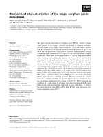
Figure 1 gives the graphical representation of the e-diagram

001226899
005664059

(10.1)
that is implicit in this “geometrical” outlook. Integers in the cells give the associated
multiplicity.
the electronic journal of combinatorics 13 (2006), #R38 20
2
1
2
1
1
1
1
Figure 1: A chessboard diagram.
The set of descents,Des(D), and the set of sign changes,Sch(D), of an e-diagram
D =

a
1

a
2
a
n
b
1
b
2
b
n

are defined to be
Des(D):={k ∈ [n − 1] | b
k
>b
k+1
and a
k
≡ a
k+1
(mod 2)},
Sch(D):={k ∈ [0,n− 1] | a
k
≡ a
k+1
(mod 2)},
where by convention a
0
≡ 1 (mod 2). In other words, 0 is in Sch(D) if and only if a
1

is
odd. Note that these two set are disjoint, i.e.,
Des(D) ∩ Sch(D)=∅.
For the e-diagram of Figure 1, we have
Des(D)={5, 6} and Sch(D)={2, 3, 7}.
We further set
g
i
(D):=2δ
i
(D)+s
i
(D), with
δ
i
(D):=#{k ∈ Des(D) | k<i}, and
s
i
(D):=#{k ∈ Sch(D) | k<i}.
Then, for any cell (a
i
,b
i
)inD,wemusthave
a
i
≥ g
i
(D). (10.2)
We now associate to each e-diagram D a signed permutation β(D) ∈ B

n
. In order to
define this β(D) we suppose that the cells of
D =

a
1
a
2
a
n
b
1
b
2
b
n

the electronic journal of combinatorics 13 (2006), #R38 21
have been ordered in increasing opposite lexicographical order. Thisissaytheorder,
denoted “≺
op
”, such that
(a, b) ≺
op
(a

,b

) ⇐⇒


b<b

or,
b = b

and a<a

.
We will call this the labelling order for cells of the diagram. Our intent here is that a
cell (a, b)ofD be labeled i,ifitsitsinD in the i
th
position with respect to this labeling
order. There is clearly a unique permutation σ such that
(a
σ(1)
,b
σ(1)
) 
lex
(a
σ(2)
,b
σ(2)
) 
lex

lex
(a
σ(n)

,b
σ(n)
),
with σ(i) <σ(j), whenever i<jand (a
i
,b
i
)=(a
j
,b
j
). We then introduce the classifying
signed permutation, β = β(D), of D, setting
β(i):=(−1)
a
i
+1
σ(i).
In this context, we often say that ≺
lex
is the reading order for the cells of D.Forthe
diagram of (10.1), represented in Figure 1, the labeling order is

008619229
000455669

.
The corresponding classifying signed permutation is readily seen to be
¯
1

¯
25
¯
7
¯
8
¯
4
¯
369.
A simple inductive argument shows that for all i’s,
g
i
(D)=g
i
(β(D)), (10.3)
justifying our use of the same notation in both cases. Now, if D =(a, b), let us set
D
∗
:= (b, a) . (10.4)
Recall that  indicates that we are passing to the associated bipartite partition. This is
to say that we are reordering the cells in increasing lex-order. It is easy to check that
β(D
∗
)=β
−1
,
if β = β(D). Thus, we naturally call D
∗
the inverse e-diagram of D. It follows from

(10.3) that
g
i
(D
∗
)=g
i
(β
−1
). (10.5)
Hence
b
i
≥ g
σ(i)
(D
∗
), (10.6)
where, as before, σ(i) is the absolute value of β(i). All this suggests that, in a manner
similar to (9.4), we use the notation
g(D):=(g
1
(D),g
2
(D), ,g
n
(D)),

g(D):=(g
1

(D), g
2
(D), ,g
n
(D)), with g
i
(D):=g
σ(i)
(D
∗
),
the electronic journal of combinatorics 13 (2006), #R38 22
where, once again, σ(i) is the absolute value of β(i). We have thus associated to each
diagram, D, a new diagram
D := (g(D),

g(D)), (10.7)
which is going to be called the compactification of D. The compact diagram associated
to (10.1) is

001224677
003442035

. (10.8)
We can check, and this will be made clear in the next Section 11, that
Proposition 10.1. For al l e-diagram D, we have
β(D)=β(
D); (10.9)
and
D = D

β
, (10.10)
with β := β(D).
We introduce an equivalence relation on the set of the e-diagrams saying that D and
˜
D are equivalent if and only if they have the same classifying signed permutation. In
symbols,
D 

D ⇐⇒ β(D)=β(

D).
In view of (9.2) the cells of D
β
are in reading order. Moreover the label of (g
i
(β), g
i
(β)) is
β(i), hence β(D
β
)=β. For the moment, the main properties of this equivalence relation
is the following.
Theorem 10.2. For any e-diagram, D, we have
β(D)=β ⇐⇒ D  D
β
.
Moreover, D
β
is minimal in the equivalence class of D, in that the matrix


D − D
β
has all entries nonnegative, for all

D  D.
The last part of this theorem is one of the reasons why we say that e-diagrams of the
form D
β
are compact. The next section will make this notion even more precise.
11 Compactification of e-diagrams
As we will currently see, compact e-diagrams D
β
can be characterized in a very sim-
ple “geometrical” manner. To obtain this characterization, we introduce the notion of
“compacting moves” for a diagram. These moves are designed to preserve the underlying
the electronic journal of combinatorics 13 (2006), #R38 23
Figure 2: Constraints on compacting moves.
classifying signed permutation. Moreover, they produce smaller diagram for the partial
order
D ≤

D.
This last statement means that the matrix

D − D only has nonnegative entries.
Now, let D be an e-diagram in which we select some cell c =(a, b), with a ≥ 2. A left
move of the cell c =(a, b)inD is defined to be

c

(D):=(D \{c}) ∪{(a − 2,b)}. (11.1)
Since it is understood here that cells are counted with multiplicities, the set difference
and union, in the right hand side of (11.1), are to be understood as multiset operations.
Thus, the result corresponds to decreasing by 1 the multiplicity of c in D, and increasing
that of (a − 2,b)by1. Now,ifc =(a, b), with b ≥ 2, a down move of the cell c =(a, b)
in D is defined to be

c
(D):=(D \{c}) ∪{(a, b − 2)}. (11.2)
Compacting moves, on a diagram D, are either left moves or down moves with some con-
straint on the choice of c as described below. A left move for c is allowed as a compacting
move if and only if the set
Vert(c, D):={c

∈ D |  (c) ≺
lex
c

≺
lex
(c)} (11.3)
is empty. Analogously, a down move for c is allowed if and only if the set
Horiz(c, D) := Vert(c
∗
,D
∗
)
∗
(11.4)
is empty. The “constraint” intervals Vert and Horiz are illustrated in Figure 2.

Observe that compacting moves do not change the sign of the cell that is moved. But
more importantly, they do not change the classifying signed permutation of the e-diagram,
namely,
D  
c
(D)  
c
(D), (11.5)
the electronic journal of combinatorics 13 (2006), #R38 24
2 1
1
1
1
2
12
¯
12 1
¯
2
¯
1
¯
2
1
1
1
1
1
1
1

1
21
¯
21 2
¯
1
¯
2
¯
1
Figure 3: Compact e-diagrams for n =2.
whenever c is so corresponds to a compacting move. The final crucial property of com-
pacting moves is that

c
(D) <D, and 
c
(D) <D. (11.6)
Diagram for which no compacting move are possible will be called compact. From (10.2)
and (10.6), it follows that the set of compact e-diagrams (see (9.3)) is exactly
{ D
β
| β ∈ B
n
}.
Observe that, starting with any given e-diagram D, if one keeps applying compacting
moves (in whatever order) until no such move is possible, then the final result will always
be the compact diagram
D. See Figure 3 for all eight compact e-diagrams associated to
elements of B

2
. In our upcoming discussion, it will be helpful to organize compacting
moves in groups, called big compacting moves. This is natural in light of the following
observation. Whenever a left compacting move is possible for a cell c =(a
i
,b
i
), then
all cells that are larger then c, in reading order, will eventually be left moved in the
compacting process. We may as well achieve all this in one step:

a
1
a
i
a
n
b
1
b
i
b
n



a
1
a
i

− 2 a
n
− 2
b
1
b
i
b
n

.
12 The bijection
The basic motivation for the introduction of compact e-diagram is the following theorem
which reflects, in combinatorial term, the bigraded module isomorphism (3.11), in the
case W = B
n
.
Theorem 12.1. There is a natural bijection, ϕ, between n-cell e-diagrams and triplets
D ↔ (
D, λ, µ),
where D is the compactification of D, and λ and µ are two partitions with parts smaller
or equal to n. Moreover, these partitions are such that
|D| = |
D| +2(|λ|, |µ|). (12.1)
the electronic journal of combinatorics 13 (2006), #R38 25