NẮM VỮNG CÁC DÃY VÀ CÔNG THỨC TRONG EXCEL – PHẦN 4 docx

NẮM VỮNG CÁC DÃY VÀ CÔNG
THỨC TRONG EXCEL – PHẦN 4

Using AutoFill to Create Text and Numeric Series
Sử dụng AutoFill để tạo ra chuỗi text và chuỗi số
Worksheets often use text series (such as January, February, March; or Sunday,
Monday, Tuesday) and numeric series (such as 1, 3, 5; or 2003, 2004, 2005).
Instead of entering these series by hand, you can use the fill handle to create them
automatically. This handy feature is called AutoFill. The following steps show you
how it works:
Các worksheet thường sử dụng chuỗi text liên tục (chẳng hạn như January,
February, March; hoặc Sunday, Monday, Tuesday) và chuỗi số liên tục (chẳng hạn
như 1, 3, 5; hoặc 2003, 2004, 2005). Thay vì nhập các chuỗi này bằng tay, bạn có
thể sử dụng fill handle để tạo chúng một cách tự động. Tính năng tiện lợi này được
gọi là AutoFill (tự động điền). Các bước sau đây hướng dẫn bạn các thực hiện điều
này:
1. For a text series, select the first cell of the range you want to use, and enter the
initial value. For a numeric series, enter the first two values and then select both
cells.
Đối với chuỗi text liên tục, bạn chọn ô đầu tiên trong dãy bạn muốn sử dụng, và
nhập cho nó một giá trị ban đầu. Đối với chuỗi số, bạn cần nhập hai giá trị đầu tiên
và rồi chọn cả hai ô.
2. Position the mouse pointer over the fill handle. The pointer changes to a plus
sign (+).
Đặt con trỏ chuột vào cái fill handle. Con trỏ chuột sẽ biến thành một dấu cộng
(+).
3. Click and drag the mouse pointer until the gray border encompasses the range
you want to fill. If you’re not sure where to stop, keep your eye on the pop-up
value that appears near the mouse pointer and shows you the series value of the
last selected cell.
Nhấp vào kéo con trỏ chuột cho đến khi có một đường viền màu xám bao quanh

dãy mà bạn muốn điền đầy. Nếu bạn không chắc chắn nơi dừng lại, bạn hãy chú ý
đến giá trị hiện lên ngay phía dưới con trỏ chuột, nó cho bạn biết giá trị của ô mà
bạn vừa kéo con trỏ chuột đi ngang qua.
4. Release the mouse button. Excel fills in the range with the series.
Nhả nút chuột ra. Excel sẽ điền đầy chuỗi liên tục vào trong dãy.
When you release the mouse button after using AutoFill, Excel not only fills in the
series, but it also displays the Auto Fill Options smart tag. To see the options,
move your mouse pointer over the smart tag and then click the downward-pointing
arrow to drop down the list. The options you see depend on the type of series you
created. However, you’ll usually see at least the following four:
Khi bạn nhả nút chuột ra sau khi sử dụng AutoFill, Excel không chỉ điền đầy vào
dãy mà còn hiển thị thêm một cái smart tag gồm những tùy chọn cho AutoFill. Để
thấy những tùy chọn này, bạn rê con trỏ chuột lên smart tag và nhấp cái mũi tên
hướng xuống để mở ra một danh sách (các tùy chọn). Những tùy chọn mà bạn thấy
phụ thuộc vào loại chuỗi mà bạn đã tạo. Tuy nhiên, thường thì bạn sẽ thấy ít nhất
có bốn tùy chọn sau đây:
Copy Cells — Click this option to fill the range by copying the original cell or
cells.
Điền đầy dãy bằng cách sao chép ô (hoặc các ô) gốc.
Fill Series — Click this option to get the default series fill.
Áp dụng một chuỗi liên tục mặc định.
Fill Formatting Only — Click this option to apply only the original cell’s
formatting to the selected range.
Chỉ áp dụng định dạng của ô gốc vào dãy được chọn.
Fill Without Formatting — Click this option to fill the range with the series data
but without the formatting of the original cell.
Điền đầy vào dãy một chuỗi liên tục, nhưng không áp dụng định dạng của ô gốc
vào dãy.
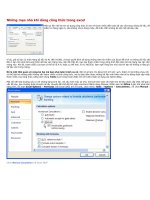
Figure 1.5 shows several series created with the fill handle (the shaded cells are
the initial fill values). Notice, in particular, that Excel increments any text value

that includes a numeric component (such as Quarter 1 and Customer 1001).
Hình 1.5 minh họa một số chuỗi được tạo bằng công cụ fill handle (các ô được tô
đậm là những giá trị ban đầu). Chú ý rằng Excel sẽ tự động gia tăng bất kỳ giá trị
text nào có một thành phần số (chẳng hạn như Quarter 1 and Customer 1001).

(Hình 1.5)
Creating a Custom AutoFill List
Tự tạo một danh sách AutoFill
As you’ve seen, Excel recognizes certain values (for example, January, Sunday,
Quarter 1) as part of a larger list. When you drag the fill handle from a cell
containing one of these values, Excel fills the cells with the appropriate series.
However, you’re not stuck with just the few lists that Excel recognized out of the
box. You’re free to define your own AutoFill lists, as described in the following
steps:
Như bạn đã thấy, Excel (tự) nhận biết (được một số) giá trị nhất định (nào đó) là
thành phần trong một danh sách (ví dụ như January, Sunday, Quarter 1). Khi bạn
kéo công cụ fill handle từ một ô chứa một trong các giá trị này, Excel sẽ điền vào
các ô (được kéo bằng fill handle) các chuỗi thích hợp. Tuy nhiên, bạn không bị
giới hạn (việc sử dụng AutoFill để điền các chuỗi liên tục cho dù) Excel chỉ nhận
biết một vài danh sách nào đó thôi. Bạn tự do định nghĩa thêm các danh sách
AutoFill của mình, theo các bước được mô tả sau đây:
1. Choose Office, Excel Options to display the Excel Options dialog box.
Chọn Office (hình tròn biểu tượng Office ở góc cao bên trái của cửa sổ bảng tính),
Excel Options để mở hộp thoại Excel Options (các tùy chọn trong Excel).
2. Click Popular and then click Edit Custom Lists to open the Custom Lists dialog
box.
Nhấp chọn Popular và rồi nhấn nút Edit Custom Lists để mở hộp thoại Custom
Lists.
3. In the Custom Lists box, click New List. An insertion point appears in the List
Entries box.

Trong khung Custom Lists, chọn mục New List. Một điểm chèn sẽ xuất hiện trong
khung List Entries.
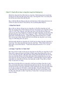
4. Type an item from your list into the List Entries box and press Enter. Repeat
this step for each item. (Make sure that you add the items in the order in which
you want them to appear in the series.) Figure 1.6 shows an example.
Nhập một từ trong danh sách (mà bạn muốn tạo) vào khung List Entries và nhấn
Enter. Lập lại bước này cho các từ khác (trong danh sách). (Hãy chắc chắn rằng
bạn thêm các mục từ theo thứ tự mà bạn muốn chúng xuất hiện trong chuỗi liên
tục.) Hình 1.6 minh họa một ví dụ:

5. Click Add to add the list to the Custom Lists box.
Nhấn nút Add để thêm danh sách (vừa tạo) vào khung Custom Lists
6. Click OK and then click OK again to return to the worksheet.
Nhấn OK hai lần để quay về worksheet.
NOTE: If you need to delete a custom list, highlight it in the Custom Lists box
and then click Delete.
Ghi chú: Nếu bạn muốn xóa một danh sách tự tạo, bạn nhấn chọn nó trong khung
Custom Lists và rồi nhấn nút Delete.
Filling a Range
Điền đầy một dãy
You can use the fill handle to fill a range with a value or formula. To do this, enter
your initial values or formulas, select them, and then click and drag the fill handle
over the destination range. (I’m assuming here that the data you’re copying won’t
create a series.) When you release the mouse button, Excel fills the range.
Bạn có thể sử dụng công cụ fill handle để điền những giá trị hoặc công thức vào
một dãy. Để thực hiện điều này, bạn nhập các giá trị hoặc công thức ban đầu, chọn
chúng, và sau đó nhấp rồi kéo công cụ fill handle cho đến hết dãy. (Ở đây, giả sử
dữ liệu ban đang sao chép sẽ không tạo ra một chuỗi liên tục). Khi bạn thả nút
chuột ra, Excel sẽ điền đầy vào dãy.
Note that if the initial cell contains a formula with relative references, Excel

adjusts the references accordingly. For example, suppose the initial cell contains
the formula =A1. If you fill down, the next cell will contain the formula =A2, the
next will contain =A3, and so on.
Lưu ý rằng, nếu ô ban đầu chứa một công thức có các tham chiếu tương đối, Excel
sẽ điều chỉnh các tham chiếu cho thích hợp. Ví dụ, ô ban đầu chứa công thức =
A1. Nếu bạn (dùng fill handle để) điền dọc xuống, ô tiếp theo sẽ chứa công thức =
A2, ô tiếp nữa sẽ chứa công thức = A3, và cứ thế mà tiếp tục