transformer engineering design and practice 1_phần 6 doc
Bạn đang xem bản rút gọn của tài liệu. Xem và tải ngay bản đầy đủ của tài liệu tại đây (632.56 KB, 42 trang )
127
4
Eddy Currents and Winding Stray
Losses
The load loss of a transformer consists of losses due to ohmic resistance of
windings (I
2
R losses) and some additional losses. These additional losses are
generally known as stray losses, which occur due to leakage field of windings and
field of high current carrying leads/bus-bars. The stray losses in the windings are
further classified as eddy loss and circulating current loss. The other stray losses
occur in structural steel parts. There is always some amount of leakage field in all
types of transformers, and in large power transformers (limited in size due to
transport and space restrictions) the stray field strength increases with growing
rating much faster than in smaller transformers. The stray flux impinging on
conducting parts (winding conductors and structural components) gives rise to
eddy currents in them. The stray losses in windings can be substantially high in
large transformers if conductor dimensions and transposition methods are not
chosen properly.
Today’s designer faces challenges like higher loss capitalization and optimum
performance requirements. In addition, there could be constraints on dimensions
and weight of the transformer which is to be designed. If the designer lowers
current density to reduce the DC resistance copper loss (I
2
R loss), the eddy loss in
windings increases due to increase in conductor dimensions. Hence, the winding
conductor is usually subdivided with a proper transposition method to minimize
the stray losses in windings.
In order to accurately estimate and control the stray losses in windings and
structural parts, in-depth understanding of the fundamentals of eddy currents
starting from basics of electromagnetic fields is desirable. The fundamentals are
described in first few sections of this chapter. The eddy loss and circulating
current loss in windings are analyzed in subsequent sections. Methods for
Copyright © 2004 by Marcel Dekker, Inc.
Chapter 4128
evaluation and control of these two losses are also described. Remaining
components of stray losses, mostly the losses in structural components, are dealt
with in Chapter 5.
4.1 Field Equations
The differential forms of Maxwell’s equations, valid for static as well as time
dependent fields and also valid for free space as well as material bodies are:
(4.1)
(4.2)
(4.3)
(4.4)
where H=magnetic field strength (A/m)
E=electric field strength (V/m)
B=flux density (wb/m
2
)
J=current density (A/m
2
)
D=electric flux density (C/m
2
)
ρ
=volume charge density (C/m
3
)
There are three constitutive relations,
J=
σ
E (4.5)
B=µ H (4.6)
D=
ε
E (4.7)
where µ=permeability of material (henrys/m)
ε
=permittivity of material (farads/m)
σ
=conductivity (mhos/m)
The ratio of the conduction current density (J) to the displacement current density
(∂D/∂t) is given by the ratio
σ
/(j
ωε
), which is very high even for a poor metallic
conductor at very high frequencies (where
ω
is frequency in rad/sec). Since our
analysis is for the (smaller) power frequency, the displacement current density is
Copyright © 2004 by Marcel Dekker, Inc.
Eddy Currents and Winding Stray Losses 129
neglected for the analysis of eddy currents in conducting parts in transformers
(copper, aluminum, steel, etc.). Hence, equation 4.2 gets simplified to
(4.8)
The principle of conservation of charge gives the point form of the continuity
equation,
(4.9)
In the absence of free electric charges in the present analysis of eddy currents in a
conductor we get
(4.10)
To get the solution, the first-order differential equations 4.1 and 4.8 involving both
H and E are combined to give a second-order equation in H or E as follows.
Taking curl of both sides of equation 4.8 and using equation 4.5 we get
For a constant value of conductivity (σ), using vector algebra the equation can be
simplified as
(4.11)
Using equation 4.6, for linear magnetic characteristics (constant µ) equation 4.3
can be rewritten as
(4.12)
which gives
(4.13)
Using equations 4.1 and 4.13, equation 4.11 gets simplified to
(4.14)
or
(4.15)
Equation 4.15 is a well-known diffusion equation. Now, in the frequency domain,
equation 4.1 can be written as follows:
(4.16)
Copyright © 2004 by Marcel Dekker, Inc.
Chapter 4130
In above equation, term j
ω
appears because the partial derivative of a sinusoidal
field quantity with respect to time is equivalent to multiplying the corresponding
phasor by j
ω
. Using equation 4.6 we get
(4.17)
Taking curl of both sides of the equation,
(4.18)
Using equation 4.8 we get
(4.19)
Following the steps similar to those used for arriving at the diffusion equation
4.15 and using the fact that (since no free
electric charges are present) we get
(4.20)
Substituting the value of J from equation 4.5,
(4.21)
Now, let us assume that the vector field E has component only along the x axis.
(4.22)
The expansion of the operator ∇ leads to the second-order partial differential
equation,
(4.23)
Suppose, if we further assume that E
x
is a function of z only (does not vary with x
and y), then equation 4.23 reduces to the ordinary differential equation
(4.24)
We can write the solution of equation 4.24 as
(4.25)
where E
xp
is the amplitude factor and
γ
is the propagation constant, which can be
given in terms of the attenuation constant
α
and phase constant
β
as
Copyright © 2004 by Marcel Dekker, Inc.
Eddy Currents and Winding Stray Losses 131
γ
=
α
+j
β
(4.26)
Substituting the value of E
x
from equation 4.25 in equation 4.24 we get
(4.27)
which gives
(4.28)
(4.29)
If the field E
x
is incident on a surface of a conductor at z=0 and gets attenuated
inside the conductor (z>0), then only the plus sign has to be taken for
γ
(which is
consistent for the case considered).
(4.30)
(4.31)
Substituting
ω
=2
π
f we get
(4.32)
Hence,
(4.33)
The electric field intensity (having a component only along the x axis and
traveling/penetrating inside the conductor in +z direction) expressed in the
complex exponential notation in equation 4.25 becomes
E
x
=E
xp
e
-
γ
z
(4.34)
which in time domain can be written as
E
x
=E
xp
e
-
α
z
cos(
ω
t-
β
z) (4.35)
Substituting the values of
α
and
β
from equation 4.33 we get
(4.36)
The conductor surface is represented by z=0. Let z>0 and z<0 represent the regions
corresponding to the conductor and perfect loss-free dielectric medium
Copyright © 2004 by Marcel Dekker, Inc.
Chapter 4132
respectively. Thus, the source field at the surface which establishes fields within
the conductor is given by
(E
x
)
z=0
=E
xp
cos
ω
t
Making use of equation 4.5, which says that the current density within a conductor
is directly related to the electrical field intensity, we can write
(4.37)
Equations 4.36 and 4.37 tell us that away from the source at the surface and with
penetration into the conductor there is an exponential decrease in the electric field
intensity and (conduction) current density. At a distance of penetration
the exponential factor becomes e
-1
(=0.368), indicating that the
value of field (at this distance) reduces to 36.8% of that at the surface. This
distance is called as the skin depth or depth of penetration
δ
,
(4.38)
All the fields at the surface of a good conductor decay rapidly as they penetrate
few skin depths into the conductor. Comparing equations 4.33 and 4.38, we getthe
relationship,
(4.39)
The depth of penetration or skin depth is a very important parameter in
describing the behavior of a conductor subjected to electromagnetic fields. The
conductivity of copper conductor at 75°C (temperature at which load loss of a
transformer is usually calculated and guaranteed) is 4.74×10
7
mhos/m. Copper
being a non-magnetic material, its relative permeability is 1. Hence, the depth of
penetration of copper at the power frequency of 50 Hz is
or 10.3 mm. The corresponding value at 60 Hz is 9.4 mm. For aluminum, whose
conductivity is approximately 61% of that of copper, the skin depth at 50 Hz is
13.2 mm. Most of the structural elements inside a transformer are made of either
mild steel or stainless steel material. For a typical grade of mild steel (MS)
material with relative permeability of 100 (assuming that it is saturated) and
conductivity of 7×10
6
mho/m, the skin depth is
δ
MS
=2.69 mm at 50 Hz. A non-
magnetic stainless steel is commonly used for structural components in the
Copyright © 2004 by Marcel Dekker, Inc.
Eddy Currents and Winding Stray Losses 133
vicinity of the field due to high currents. For a typical grade of stainless steel (SS)
material with relative permeability of 1 (non-magnetic) and conductivity of
1.136×10
6
mho/m, the skin depth is
δ
ss
=66.78 mm at 50 Hz.
4.2 Poynting Vector
Poynting’s theorem is the expression of the law of conservation of energy applied
to electromagnetic fields. When the displacement current is neglected, as in the
previous section, Poynting’s theorem can be mathematically expressed as [1,2]
(4.40)
where v is the volume enclosed by the surface s and n is the unit vector normal to
the surface directed outwards. Using equation 4.5, the above equation can be
modified as,
(4.41)
This is a simpler form of Poynting’s theorem which states that the net inflow of
power is equal to the sum of the power absorbed by the magnetic field and the
ohmic loss. The Poynting vector is given by the vector product,
P=E×H (4.42)
which expresses the instantaneous density of power flow at a point.
Now, with E having only the x component which varies as a function of z only,
equation 4.17 becomes
(4.43)
Substituting the value of E
x
from equation 4.34 and rearranging we get
(4.44)
The ratio of E
x
to H
y
is defined as the intrinsic impedance,
(4.45)
Substituting the value of
γ
from equation 4.30 we get
Copyright © 2004 by Marcel Dekker, Inc.
Chapter 4134
(4.46)
Using equation 4.38, the above equation can be rewritten as
(4.47)
Now, equation 4.36 can be rewritten in terms of skin depth as
E
x
=E
xp
e
-z/δ
cos(
ω
t-z/
δ
) (4.48)
Using equations 4.45 and 4.47, H
y
can be expressed as
(4.49)
Since E is in the x direction and H is in the y direction, the Poynting vector, which
is a cross product of E and H as per equation 4.42, is in the z direction.
(4.50)
Using the identity cosA cosB=1/2[cos(A+B)+cos(A-B)], the above equation
simplifies to
(4.51)
The time average Poynting vector is then given by
(4.52)
Thus, it can be observed that at a distance of one skin depth (z=
δ
), the power
density is only 0.135 (=e
-2
) times its value that at the surface. This is very
important fact for the analysis of eddy currents and losses in structural
components of transformers. If the eddy losses in the tank of a transformer due to
incident leakage field emanating from windings are being analyzed by using FEM
analysis, then there should be at least two or three elements in one skin depth for
getting accurate results.
Let us now consider a conductor with field E
xp
and the corresponding current
density J
xp
at the surface as shown in figure 4.1. The fields have the value of 1 p.u.
Copyright © 2004 by Marcel Dekker, Inc.
Eddy Currents and Winding Stray Losses 135
at the surface. The total power loss in height (length) h and width b is given by the
value of power crossing the conductor surface [2] within the area (h ×b),
(4.53)
The total current in the conductor is found out by integrating the current density
over the infinite depth of the conductor. Using equations 4.34 and 4.39 we get
(4.54)
If this total current is assumed to be uniformly distributed in one skin depth, the
uniform current density can be expressed in the time domain as
(4.55)
Figure 4.1 Penetration of field inside a conductor
Copyright © 2004 by Marcel Dekker, Inc.
Chapter 4136
The total ohmic power loss is given by
(4.56)
The average value of power can be found out as
(4.57)
Since the average value of a cosine term over integral number of periods is zero we
get
(4.58)
which is the same as equation 4.53. Hence, the average power loss in a conductor
may be computed by assuming that the total current is uniformly distributed in one
skin depth. This is a very important result, which is made use of in calculation of
eddy current losses in conductors by numerical methods. When a numerical
method such as Finite Element Method (FEM) is used for estimation of stray
losses in the tank (made of mild steel) of a transformer, it is important to have
element size less than the skin depth of the tank material as explained earlier. With
the other transformer dimensions in meters, it is difficult to have very small
elements inside the tank thickness. Hence, it is convenient to use analytical results
to simplify the numerical analysis. For example in [3], equation 4.58 is used for
estimation of tank losses by 3-D FEM analysis. The method assumes uniform
current density in the skin depth allowing the use of relatively larger element sizes.
The above-mentioned problem of modeling and analysis of skin depths can
also be taken care by using the concept of surface impedance. The intrinsic
impedance can be rewritten from equation 4.46 as
(4.59)
The real part of the impedance, termed as surface resistance, is given by
(4.60)
After calculating the r.m.s. value of the tangential component of the magnetic field
intensity (H
rms
) at the surface of the tank or any other structural component in the
transformer by either numerical or analytical method, the specific loss per unit
surface area can be calculated by the expression [4,5]
Copyright © 2004 by Marcel Dekker, Inc.
Eddy Currents and Winding Stray Losses 137
(4.61)
Thus, the total losses in the transformer tank can be determined by integrating the
specific loss on its internal surface.
4.3 Eddy Current and Hysteresis Losses
All the analysis done previously assumed linear material (B-H) characteristics
meaning that the permeability (µ) is constant. The material used for structural
components in transformers is usually magnetic steel (mild steel), which is a
ferromagnetic material having a much larger value of relative permeability (µ
r
) as
compared to the free space (for which µ
r
=1). The material has non-linear B-H
characteristics and the permeability itself is a function of H. Moreover, the
characteristics also exhibit hysteresis property. Equation 4.6 (B=µH)has to be
suitably modified to reflect the non-linear characteristics and hysteresis behavior.
Hysteresis introduces a time phase difference between B and H; B lags H by an
angle (
θ
) known as the hysteresis angle. One of the ways in which the
characteristics can be mathematically expressed is by complex or elliptical
permeability,
µ
h
=µe
-j
θ
(4.62)
In this formulation, where harmonics introduced by saturation are ignored, the
hysteresis loop becomes an ellipse with the major axis making an angle of
θ
with
the H axis as shown in figure 4.2. The significance of complex permeability is that
a functional relationship between B and H is now realized in which the
permeability is made independent of H resulting into a linear system [6]. Let us
now find an expression for the eddy current and hysteresis loss for an infinite half-
space shown in figure 4.3.
Figure 4.2 Elliptic hysteresis loop Figure 4.3 Infinite half space
Copyright © 2004 by Marcel Dekker, Inc.
Chapter 4138
The infinite half-space is an extension of the geometry shown in figure 4.1 in the
sense that the region of the material under consideration extends from -∞ to +∞ in
the x and y directions, and from 0 to ∞ in the z direction. Similar to Section 4.1, we
assume that E and H vectors have components in only the x and y directions
respectively, and that they are function of z only. The diffusion equation 4.15 can
be rewritten for this case with the complex permeability as
(4.63)
A solution satisfying boundary conditions,
H
y
=H
0
at z=0 and H
y
=0 at z=∞ (4.64)
is given by
H
y
=H
0
e
-kz
(4.65)
where constant k is
(4.66)
and
α
=cos(
θ
/2)+sin(
θ
/2) and
β
=cos(
θ
/2)-sin(
θ
/2) (4.67)
(4.68)
Using equation 4.8 and the fact that H
x
=H
z
=0 we get
(4.69)
The time average density of eddy and hysteresis losses can be found by computing
the real part of the complex Poynting vector evaluated at the surface [1],
(4.70)
Now,
(4.71)
and
(4.72)
(4.73)
Copyright © 2004 by Marcel Dekker, Inc.
Eddy Currents and Winding Stray Losses 139
In the absence of hysteresis (
θ
=0),
α
=
β
=1 as per equation 4.67. Hence, the eddy
loss per unit surface area is given by
(4.74)
Substituting the expression for skin depth from equation 4.38 and using the r.m.s.
value of magnetic field intensity (H
rms
) at the surface we get
(4.75)
which is same as equation 4.61, as it should be in the absence of hysteresis (for
linear B-H characteristics).
4.4 Effect of Saturation
In a transformer, the structural components (mostly made from magnetic steel) are
subjected to the leakage field and/or high current field. The incident field gets
predominantly concentrated in the skin depth (1 to 3 mm) near the surface. Hence,
the structural components may be in a state of saturation depending upon the
magnitude of the incident field. The eddy current losses predicted by the
calculations based on a constant relative permeability are found to be smaller than
the actual experimental values. Thus, although the magnetic saturation is part of
same physical phenomenon as the hysteresis effect, it is considerably more
important in its effect on the eddy current losses. The step function magnetization
curve, as shown in figure 4.4 (a), is the simplest way of taking the saturation into
account for an analytical solution of eddy current problems. It can be expressed by
an equation,
Figure 4.4 Step-magnetization
Copyright © 2004 by Marcel Dekker, Inc.
Chapter 4140
B=(sign of H)B
s
(4.76)
where B
s
is the saturation flux density. The magnetic field intensity H at the
surface is sinusoidally varying with time (=H
0
sin
ω
t). The extreme depth to which
the field penetrates and beyond which there is no field is called as depth of
penetration
δ
s
. This depth of penetration has a different connotation as compared
to that with constant or linear permeability. In this case, the depth of penetration is
simply the maximum depth the field will penetrate at the end of each half period.
The depth of penetration for a thick plate (thickness much larger than the depth of
penetration so that it can be considered as infinite half space) is given by [1,7,8]
(4.77)
It can be observed that for this non-linear case with step magnetization
characteristics, the linear permeability in equation 4.38 gets replaced by the ratio
B
s
/H
0
. Further, the equation for average power per unit area can be derived as
(478)
Comparing this with equation 4.74, it can be noted that if we put µ=B
s
/H
0
,
δ
s
will
be equal to
δ
and in that case the loss in the saturated material is 70% higher than
the loss in the material having linear B-H characteristics. Practically, the actual B-
H curve is in between the linear and step characteristics, as shown in figure 4.4 (b).
In [7], it is pointed out that as we penetrate inside into the material, each
succeeding inner layer is magnetized by a progressively smaller number of
exciting ampere-turns because of shielding effect of eddy currents in the region
between the outermost surface and the layer under consideration. In step-
magnetization characteristics, the flux density has the same magnitude
irrespective of the magnitude of mmf. Due to this departure of the step curve
response from the actual response, the value of B
s
is replaced by 0.75×B
s
. From
equations 4.77 and 4.78, it is clear that and hence the constant 1.7 in
equation 4.78 would reduce to i.e., 1.47. As per Rosenberg’s theory,
the constant is 1.33 [7]. Hence, in the simplified analytical formulations, linear
characteristics are assumed after taking into account the non-linearity by the
linearization coefficient in the range of 1.3 to 1.5. For example, a coefficient of 1.4
is used in [9] for the calculation of losses in tank and other structural components
in transformers.
After having seen in details the fundamentals of eddy currents, we will now
analyze eddy current and circulating current losses in windings in the following
sections. Analysis of stray losses in structural components, viz. tank, frames, flitch
plates, high current terminations, etc., is covered in Chapter 5.
Copyright © 2004 by Marcel Dekker, Inc.
Eddy Currents and Winding Stray Losses 141
4.5 Eddy Loss in Transformer Winding
4.5.1 Expression for eddy loss
Theory of eddy currents explained in the previous sections will be useful while
deriving the expression for the eddy loss in windings. The losses in a transformer
winding due to an alternating current are usually more than that due to direct
current of the same effective (r.m.s.) value. There are two different approaches of
analyzing this increase in losses. In the first approach, we assume that the load
current in the winding is uniformly distributed in the conductor cross section
(similar to the direct current) and, in addition to the load current, there exist eddy
currents which produce extra losses. Alternatively, one can calculate losses due to
the combined action of the load current and eddy currents. The former method is
more suitable for the estimation of eddy loss in winding conductors, in which
eddy loss due to the leakage field (produced by the load current) is calculated
separately and then added to the DC I
2
R loss. The latter method is preferred for
calculating circulating current losses, in which the resultant current in each
conductor is calculated first, followed by the calculation of losses (which give the
total of DC I
2
R loss and circulating current loss). We will first analyze eddy losses
in windings in this section; the circulating current losses are dealt with in the next
section.
Consider a winding conductor, as shown in figure 4.5, which is placed in an
alternating magnetic field along the y direction having the peak amplitude of H
0
.
The conductor can be assumed to be infinitely long in the x direction. The current
density J
x
and magnetic field intensity H
y
are assumed as functions of z only.
Rewriting the (diffusion) equation 4.15 for the sinusoidal variation of the field
quantity and noting that the winding conductor, either copper or aluminum, has
constant permeability (linear B-H characteristics),
(4.79)
Figure 4.5 Estimation of eddy loss in a winding conductor
Copyright © 2004 by Marcel Dekker, Inc.
Chapter 4142
A solution satisfying this equation is
H
y
=C
1
e
γ
z
+C
2
e
-
γ
z
(4.80)
where
γ
is defined by equation 4.32. In comparison with equation 4.65, equation
4.80 has two terms indicating waves traveling in both +z and -z directions (which
is consistent with figure 4.5). The incident fields on both the surfaces, having peak
amplitude of H
0
, penetrate inside the conductor along the z axis in opposite
directions (it should be noted that equation 4.80 is also a general solution of
equation 4.63, in which case C
1
=0 and C
2
=H
0
for the boundary conditions
specified by equation 4.64). For the present case, the boundary conditions are
H
y
=H
0
at z=+b and H
y
=H
0
at z=-b (4.81)
Using these boundary conditions, we can get the expression for the constants as
(4.82)
Putting these values of constants in equation 4.80 we get
(4.83)
Using equation 4.8 and the fact that H
x
=H
z
=0, the current density is
(4.84)
The loss produced per unit surface area (of the x-y plane) of the conductor in terms
of the peak value of current density is given by
(4.85)
Now, using equation 4.39 we get
Copyright © 2004 by Marcel Dekker, Inc.
Eddy Currents and Winding Stray Losses 143
Substituting this magnitude of current density in equation 4.85 we get
(4.87)
(4.88)
or
(4.89)
where
When equation 4.89 can be simplified to
(4.90)
Equation 4.90 gives the value of eddy loss per unit surface area of a conductor
with its dimension, perpendicular to the applied field, much greater than the depth
of penetration. Such a case, with the field applied on both the surfaces of the
conductor, is equivalent to two infinite half spaces. Therefore, the total eddy loss
given by equation 4.90 is two times that of the infinite half space given by
equation 4.74. For such thick conductors/plates (winding made of copper bars,
(4.86)
Copyright © 2004 by Marcel Dekker, Inc.
Chapter 4144
Neglecting higher order terms and substituting the expression of
δ
from equation
4.38 we get
(4.92)
Now, if the thickness of the winding conductor is t, then substituting b=t/2 in
equation 4.92 we get
(4.93)
It is more convenient to find an expression for the mean eddy loss per unit volume
(since the volume of the conductor in the winding is usually known). Hence,
dividing by t and finally substituting resistivity (
ρ
) in place of conductivity, we get
the expression for the eddy loss in the winding conductor per unit volume as
(4.94)
In case of thin conductors, the eddy currents are restricted by the lack of space or
high resistivity and are said to be resistance limited. In other words, since the field
of the eddy currents is negligible for thin conductors, the behavior is resistance
structural component made of magnetic steel having sufficiently large thickness,
etc.), the resultant current distribution is greatly influenced and limited by the
effect its own field and the currents are said to be inductance limited (currents are
confined to the surface layers).
Now, let us analyze the case when dimension (thickness) of the conductor is
quite small as compared to its depth of penetration, which is usually the case for
rectangular paper insulated conductors used in transformers. For 2b<<
δ
, i.e.,
ξ
<<1, equation 4.89 can be simplified to
(4.91)
Copyright © 2004 by Marcel Dekker, Inc.
Eddy Currents and Winding Stray Losses 145
limited. Equation 4.94 matches exactly with that derived in [10] by ignoring the
magnetic field produced by the eddy currents. These currents are 90° out of phase
with the load current (uniformly distributed current which produces the leakage
field and is also responsible for DC I
2
R loss in windings) flowing in the conductor.
The eddy currents are shown to be lagging by 90° with respect to the load (source)
current for a thin circular conductor in the later part of this section. The total
current flowing in the conductor can be visualized to be a vector sum of the eddy
current (I
eddy
) and load current (I
load
), having the magnitude of
because these two current components are 90° out of phase in a thin conductor.
This is a very important and convenient result because it means that the I
2
R losses
due to load current and eddy current losses can be calculated separately and then
added later for thin conductors.
Equation 4.94 is very well-known and useful formula for calculation of eddy
losses in windings. If we assume that the leakage field in windings is in axial
direction only, then we can calculate the mean value of eddy loss in the whole
winding by using the equations of Section 3.1.1. The axial leakage field for an
inner winding (with a radial depth of R and height of H
W
) varies linearly from
inside diameter to outside diameter as shown in figure 4.6. The thickness of the
conductor, which is its dimension perpendicular to the axial field, is usually quite
small. Hence, the same value of flux density (B
0
) can be assumed along both its
vertical surfaces (along width w). The position of the conductor changes along the
radial depth as the turns are wound. Hence, in order to calculate the mean value of
the eddy loss of the whole winding, we have to first calculate the mean value of
The r.m.s. value of ampere turns are linearly changing from 0 at the inside
diameter (ID) to NI at the outside diameter (OD). The peak value of flux density at
a distance x from the inside diameter is
(4.95)
The mean flux density value, which gives the same overall loss, is given by
(4.96)
Simplifying we get
(4.97)
Copyright © 2004 by Marcel Dekker, Inc.
Chapter 4146
where B
gp
is the peak value of flux density in the LV-HV gap,
(4.98)
Hence, using equations 4.97 and 4.94, the mean eddy loss per unit volume of the
winding due to the axial leakage field is expressed as
(4.99)
If we are interested in finding the mean value of eddy loss in a section of a
winding in which ampere-turns are changing from
α
(NI) at ID to b(NI) at OD,
where NI are rated r.m.s. ampere-turns, the mean value of can be easily found
out by using the procedure similar to that given in Section 3.1.1 as
(4.100)
and the mean eddy loss per unit volume in the section is
(4.101)
Equation 4.101 tells us that for a winding consisting of a number of layers, the
mean eddy loss of the layer adjacent to LV-HV gap is higher than that of others.
For example, in the case of a 2-layer winding,
Figure 4.6 Leakage flux density in winding
Copyright © 2004 by Marcel Dekker, Inc.
Eddy Currents and Winding Stray Losses 147
indicating that the mean eddy loss in the second layer close to the gap is 1.75
times the mean eddy loss for the entire winding. Similarly, for a 4-layer winding,
giving the mean eddy loss in the 4
th
layer as 2.31 times the mean eddy loss for the
entire winding. Hence, it is always advisable to calculate the total loss (I
2
R+eddy)
in each layer separately and estimate the temperature rise of each layer. Such a
calculation procedure helps designers to take countermeasures to eliminate high
temperature rise in windings. Also, the temperatures measured by fiber-optic
sensors (if installed) will be closer to the calculated values when such a calculation
procedure is adopted.
Eddy loss calculated by equation 4.99 is approximate since it assumes the
leakage field entirely in the axial direction. As seen in Chapter 3, there exists a
radial component of the leakage field at winding ends and in winding zones where
ampere-turns per unit height are different for LV and HV windings. For small
distribution transformers, the error introduced by neglecting the radial field may
not be appreciable, and equation 4.99 is generally used with some empirical
correction factor applied to the total calculated stray loss value. Analytical/
numerical methods, described in Chapter 3, need to be used for the correct
estimation of the radial field. The amount of efforts required for getting the
accurate eddy loss value may not get justified for very small distribution
transformers. For medium and large power transformers, however, the eddy loss
due to the radial field has to be estimated and the same can be found out by using
equation 4.94, for which the dimension of the conductor perpendicular to the
radial field is its width w. Hence, the eddy losses per unit volume due to axial (B
y
)
and radial (B
x
) components of leakage field are
(4.102)
(4.103)
Thus, the leakage field incident on a winding conductor (see figure 4.7) is
resolved into two components, viz. B
y
and B
x
, and losses due to these two
Copyright © 2004 by Marcel Dekker, Inc.
Chapter 4148
components are calculated separately by equations 4.102 and 4.103 and then
added. This is permitted because the eddy currents associated with these two
perpendicular components do not overlap (since the angle between them is 90°).
We have assumed that the conductor dimension is very much less than the
depth of penetration while deriving equation 4.94. This is particularly true in the
case of loss due to the axial field. The conductor thickness used in transformers
mostly falls in the range of 2 to 3.5 mm, which is considerably less than the depth
of penetrations of copper and aluminum which are 10.3 mm and 13.2 mm
respectively at 50 Hz. The conductor width is usually closer to the value of depth
of penetration. If the conductor width is equal to the depth of penetration
(w=2b=
δ
), equation 4.89 becomes
Comparing this value with that given by equation 4.92,
the error of just 4% is obtained, which is quite acceptable. Hence, it can be
concluded that the eddy loss due to the radial field can also be calculated with a
reasonable accuracy from equation 4.103 for the conductor widths comparable to
the depth of penetration.
For thin circular conductors of radius of R, if the ratio R/
δ
is small, we can
neglect the magnetic field of eddy currents. If the total current in the conductor is
I cos
ω
t, the uniform current density is given by
(4.104)
Figure 4.7 Winding conductor in a leakage field
Copyright © 2004 by Marcel Dekker, Inc.
Eddy Currents and Winding Stray Losses 149
and the eddy current density at any radius r inside the conductor is [8]
(4.105)
Thus, it can be observed from equations 4.104 and 4.105 that for thin
conductors (resistance-limited behavior), the eddy currents lag the exciting
current (the current which produces the field responsible for eddy currents) by
90°. Contrary to this, for thick conductors (thickness or radius much larger than
the depth of penetration), the eddy currents lag the exciting current by 180°
(inductance-limited behavior in which the currents are confined to the surface
layers).
The power loss per unit length of the thin circular conductor can be found out
by using equations 4.104 and 4.105 as (J
0
and J
e
are 90° apart, square of their sum
is sum of their squares)
(4.106)
The power loss per unit length due to the exciting current alone is
(4.107)
Therefore, the ratio of effective AC resistance to DC resistance of a thin circular
conductor can be deduced from equations 4.106 and 4.107 as
(4.108)
For thick circular conductors (R>>
δ
), the effective resistance is that of the
annular ring of diameter 2R and thickness
δ
, since all the current can be assumed
to be concentrated in one depth of penetration as seen in Section 4.2. Hence, the
effective AC resistance per unit length is
R
AC
=1/(2
π
R
δσ
) (4.109)
and
(4.110)
4.5.2 Methods of estimation
As said earlier, the axial and radial components of a field can be estimated by
analytical or numerical methods. Accurate estimation of eddy loss due to the
Copyright © 2004 by Marcel Dekker, Inc.
Chapter 4150
radial leakage field by means of empirical formulae is not possible. The analytical
methods [11,12] and two-dimensional FEM [13, 14] can be used to calculate the
eddy loss due to axial and radial leakage fields. It is assumed that the eddy currents
do not have influence on the leakage field (the case of thin conductors). The FEM
analysis is quite commonly used for the eddy loss calculations. The winding is
divided into many sections. For each section the corresponding ampere-turn
density is defined. The value of conductivity is not defined for these sections. The
values of B
y
and B
x
for each conductor can be obtained from the FEM solution, and
then the axial and radial components of the eddy loss are calculated for each
conductor by using equations 4.102 and 4.103 respectively. The B
y
and B
x
values
are assumed to be constant over a single conductor and equal to the value at the
center of the conductor. If the cylindrical coordinate system is used, B
y
and B
x
components are replaced by B
z
and B
r
components respectively. The total eddy
loss for each winding is calculated by integrating the loss components of all its
conductors.
Sometimes a very quick but reasonably accurate calculation of eddy loss is
required. At the tender design stage, an optimization program may have to work
hundreds of designs to arrive at the optimum design. In such cases, expressions for
the eddy loss in windings for their simple configurations can be found out using
multiple regression method in conjunction with Orthogonal Array Design of
Experiments technique [15]. With the quantum improvement in the speed of
computational tools, it is now possible to integrate the accurate analytical/
numerical methods in the main design optimization program.
For cylindrical windings in core-type transformers, the two-dimensional
methods give sufficiently accurate eddy loss values. For getting most accurate
results, three-dimensional magnetic field calculations have also been used [16,
17,18]. Once the three-dimensional field solution is obtained, the three
components of the flux density (B
x
, B
y
and B
z
) are resolved into two components,
viz. the axial and radial components, which enables the use of equations 4.102 and
4.103 for the eddy loss evaluation.
For small distribution transformers with LV winding having crossmatic
conductor (thick rectangular bar conductor), each and every turn of LV winding
has to be modeled (with the value of conductivity defined) in FEM analysis. This
is because the thickness of the bar conductor is usually comparable to or
sometimes more than the depth of penetration and its width is usually more than 5
times the depth of penetration. With such a conductor having large dimensions, a
significant modification of the leakage field occurs due to the eddy currents,
which cannot be neglected in the calculations.
The problem of accurate estimation of winding eddy loss seems to be quite
resolved by method such as 2-D FEM. The analysis of winding eddy loss by 3-D
FEM analysis is the most accurate one, but the computational efforts involved
should be compared with the improvement obtained in the accuracy.
Copyright © 2004 by Marcel Dekker, Inc.
Eddy Currents and Winding Stray Losses 151
4.5.3 Optimization of losses and elimination of winding hot spots
In order to reduce the DC resistance (I
2
R) loss, if the designer increases the
conductor dimensions, the eddy loss in windings increases. Hence, optimization
of the total of I
2
R and eddy loss should be done.
The knowledge of flux density distribution in a winding helps in choosing
proper dimensions of conductors. This is particularly important for a winding with
tappings within its body, in which the high value of radial flux density can cause
excessive loss and temperature rise. For the minimization of radial flux, balancing
of ampere-turns per unit height of LV and HV windings should be done (for
various sections along their height) at the average tap position. The winding can
be designed with different conductor dimensions in the tap zone to minimize the
risk of hot spots. Guidelines are given in [19] for choosing the conductor width for
eliminating hot spots in windings. For 50 Hz frequency, the maximum width that
can be used is usually in the range of 12 to 14 mm, whereas for 60 Hz it is of the
order of 10 to 12 mm. This guideline is useful in the absence of detailed analysis
which involves calculation of temperature rise in the part of the winding where a
hot spot is expected. For calculating the temperature rise of a disk/turn, its I
2
R loss
and eddy loss should be added. An idle winding between LV and HV windings
links the high gap flux resulting in higher eddy loss. Hence, its conductor
dimensions should be properly decided.
In gapped core shunt reactors, there is considerable flux fringing between limb
packets (separated by non-magnetic gap), resulting in an appreciable radial flux
causing excessive losses in the reactor winding if the distance between the reactor
winding and core is small or if the conductor width is large.
One of the most logical ways of reducing the eddy loss of a winding is to sub-
divide winding conductors into a number of parallel conductors. If a conductor
having thickness t is sub-divided into 2 insulated parallel conductors of thickness
t/2, the eddy loss due to axial leakage field reduces by a factor of 1/4 (refer to
equation 4.102). In actual practice, from the short circuit withstand considerations
there is a limitation imposed on the minimum thickness that can be used. Also, if
the width to thickness ratio of a rectangular conductor is more than about 6, there
is difficulty in winding it. The sub-division of the conductor also impairs the
winding space factor in the radial direction. This is because each individual
parallel conductor in a turn has to be insulated increasing the total insulation
thickness in the radial direction. In order to improve the space factor, sometimes a
bunch conductor is used in which usually two or three parallel conductors are
bunched in a common paper covering. The advantage is that the individual
conductor needs to be insulated with a lower paper insulation thickness because of
the outermost common paper covering. A single bunch conductor is also easier to
wind, since no crossovers are required at ID and OD of the winding. In contrast to
this, for example in the case of two parallel conductors, the two conductors are
usually crossed over at ID and OD of each disk for the ease of winding. Three
rectangular strip conductors and the corresponding bunch conductor are shown in
Copyright © 2004 by Marcel Dekker, Inc.