Computer organization and design Design 2nd phần 2 pptx

2.5 Type and Size of Operands 85
Summary: Operations in the Instruction Set
From this section we see the importance and popularity of simple instructions:
load, store, add, subtract, move register-register, and, shift, compare equal, com-
pare not equal, branch, jump, call, and return. Although there are many options
for conditional branches, we would expect branch addressing in a new architec-
ture to be able to jump to about 100 instructions either above or below the branch,
implying a PC-relative branch displacement of at least 8 bits. We would also ex-
pect to see register-indirect and PC-relative addressing for jump instructions to
support returns as well as many other features of current systems.
How is the type of an operand designated? There are two primary alternatives:
First, the type of an operand may be designated by encoding it in the opcode—
this is the method used most often. Alternatively, the data can be annotated with
tags that are interpreted by the hardware. These tags specify the type of the oper-
and, and the operation is chosen accordingly. Machines with tagged data, howev-
er, can only be found in computer museums.
Usually the type of an operand—for example, integer, single-precision float-
ing point, character—effectively gives its size. Common operand types include
character (1 byte), half word (16 bits), word (32 bits), single-precision floating
point (also 1 word), and double-precision floating point (2 words). Characters are
almost always in ASCII and integers are almost universally represented as two’s
complement binary numbers. Until the early 1980s, most computer manufactur-
ers chose their own floating-point representation. Almost all machines since that
time follow the same standard for floating point, the IEEE standard 754. The
IEEE floating-point standard is discussed in detail in Appendix A.
Some architectures provide operations on character strings, although such op-
erations are usually quite limited and treat each byte in the string as a single char-
acter. Typical operations supported on character strings are comparisons and
moves.
For business applications, some architectures support a decimal format, usu-
ally called packed decimal or binary-coded decimal

;—4 bits are used to encode
the values 0–9, and 2 decimal digits are packed into each byte. Numeric character
strings are sometimes called unpacked decimal, and operations—called packing
and unpacking—are usually provided for converting back and forth between
them.
Our benchmarks use byte or character, half word (short integer), word (inte-
ger), and floating-point data types. Figure 2.16 shows the dynamic distribution of
the sizes of objects referenced from memory for these programs. The frequency
of access to different data types helps in deciding what types are most important
to support efficiently. Should the machine have a 64-bit access path, or would
2.5
Type and Size of Operands
86 Chapter 2 Instruction Set Principles and Examples
taking two cycles to access a double word be satisfactory? How important is it to
support byte accesses as primitives, which, as we saw earlier, require an alignment
network? In Figure 2.16, memory references are used to examine the types of data
being accessed. In some architectures, objects in registers may be accessed as
bytes or half words. However, such access is very infrequent—on the VAX, it ac-
counts for no more than 12% of register references, or roughly 6% of all operand
accesses in these programs. The successor to the VAX not only removed opera-
tions on data smaller than 32 bits, it also removed data transfers on these smaller
sizes: The first implementations of the Alpha required multiple instructions to read
or write bytes or half words.
Note that Figure 2.16 was measured on a machine with 32-bit addresses: On a
64-bit address machine the 32-bit addresses would be replaced by 64-bit address-
es. Hence as 64-bit address architectures become more popular, we would expect
that double-word accesses will be popular for integer programs as well as float-
ing-point programs.
Summary: Type and Size of Operands
From this section we would expect a new 32-bit architecture to support 8-, 16-,

and 32-bit integers and 64-bit IEEE 754 floating-point data; a new 64-bit address
architecture would need to support 64-bit integers as well. The level of support
for decimal data is less clear, and it is a function of the intended use of the ma-
chine as well as the effectiveness of the decimal support.
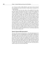
FIGURE 2.16 Distribution of data accesses by size for the benchmark programs. Ac-
cess to the major data type (word or double word) clearly dominates each type of program.
Half words are more popular than bytes because one of the five SPECint92 programs (eqn-
tott) uses half words as the primary data type, and hence they are responsible for 87% of the
data accesses (see Figure 2.31 on page 110). The double-word data type is used solely for
double-precision floating-point in floating-point programs. These measurements were taken
on the memory traffic generated on a 32-bit load-store architecture.
0%
40% 80%20% 60%
0%
19%
7%
31%
74%
Word
Half word
Byte
0%
0%
Double word
69%
Frequency of reference by size
Integer average Floating-point average
2.6 Encoding an Instruction Set 87
Clearly the choices mentioned above will affect how the instructions are encoded
into a binary representation for execution by the CPU. This representation affects

not only the size of the compiled program, it affects the implementation of the
CPU, which must decode this representation to quickly find the operation and its
operands. The operation is typically specified in one field, called the opcode. As
we shall see, the important decision is how to encode the addressing modes with
the operations.
This decision depends on the range of addressing modes and the degree of in-
dependence between opcodes and modes. Some machines have one to five oper-
ands with 10 addressing modes for each operand (see Figure 2.5 on page 75). For
such a large number of combinations, typically a separate address specifier is
needed for each operand: the address specifier tells what addressing mode is used
to access the operand. At the other extreme is a load-store machine with only one
memory operand and only one or two addressing modes; obviously, in this case,
the addressing mode can be encoded as part of the opcode.
When encoding the instructions, the number of registers and the number of ad-
dressing modes both have a significant impact on the size of instructions, since the
addressing mode field and the register field may appear many times in a single in-
struction. In fact, for most instructions many more bits are consumed in encoding
addressing modes and register fields than in specifying the opcode. The architect
must balance several competing forces when encoding the instruction set:
1. The desire to have as many registers and addressing modes as possible.
2. The impact of the size of the register and addressing mode fields on the aver-
age instruction size and hence on the average program size.
3. A desire to have instructions encode into lengths that will be easy to handle in
the implementation. As a minimum, the architect wants instructions to be in
multiples of bytes, rather than an arbitrary length. Many architects have cho-
sen to use a fixed-length instruction to gain implementation benefits while sac-
rificing average code size.
Since the addressing modes and register fields make up such a large percent-
age of the instruction bits, their encoding will significantly affect how easy it is
for an implementation to decode the instructions. The importance of having easi-

ly decoded instructions is discussed in Chapter 3.
Figure 2.17 shows three popular choices for encoding the instruction set. The
first we call variable, since it allows virtually all addressing modes to be with all
operations. This style is best when there are many addressing modes and opera-
tions. The second choice we call fixed, since it combines the operation and the
2.6
Encoding an Instruction Set
88 Chapter 2 Instruction Set Principles and Examples
addressing mode into the opcode. Often fixed encoding will have only a single
size for all instructions; it works best when there are few addressing modes and
operations. The trade-off between variable encoding and fixed encoding is size of
programs versus ease of decoding in the CPU. Variable tries to use as few bits as
possible to represent the program, but individual instructions can vary widely in
both size and the amount of work to be performed. For example, the VAX integer
add can vary in size between 3 and 19 bytes and vary between 0 and 6 in data
memory references. Given these two poles of instruction set design, the third al-
ternative immediately springs to mind: Reduce the variability in size and work of
the variable architecture but provide multiple instruction lengths so as to reduce
code size. This hybrid approach is the third encoding alternative.
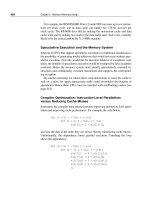
FIGURE 2.17 Three basic variations in instruction encoding. The variable format can
support any number of operands, with each address specifier determining the addressing
mode for that operand. The fixed format always has the same number of operands, with the
addressing modes (if options exist) specified as part of the opcode (see also Figure C.3 on
page C-4). Although the fields tend not to vary in their location, they will be used for different
purposes by different instructions. The hybrid approach will have multiple formats specified
by the opcode, adding one or two fields to specify the addressing mode and one or two fields
to specify the operand address (see also Figure D.7 on page D-12)
.
Operation &
no. of operands

Address
specifier 1
Address
field 1
Address
field 1
Operation Address
field 2
Address
field 3
Address
specifier
Operation Address
field
Address
specifier 1
Operation Address
specifier 2
Address
field
Address
specifier
Operation Address
field 1
Address
field 2
Address
specifier n
Address
field n

(a) Variable (e.g., VAX)
(b) Fixed (e.g., DLX, MIPS, Power PC, Precision Architecture, SPARC)
(c) Hybrid (e.g., IBM 360/70, Intel 80x86)
2.7 Crosscutting Issues: The Role of Compilers 89
To make these general classes more specific, this book contains several exam-
ples. Fixed formats of five machines can be seen in Figure C.3 on page C-4 and
the hybrid formats of the Intel 80x86 can be seen in Figure D.8 on page D-13.
Let’s look at a VAX instruction to see an example of the variable encoding:
addl3 r1,737(r2),(r3)
The name addl3 means a 32-bit integer add instruction with three operands, and
this opcode takes 1 byte. A VAX address specifier is 1 byte, generally with the
first 4 bits specifying the addressing mode and the second 4 bits specifying the
register used in that addressing mode. The first operand specifier—r1—indicates
register addressing using register 1, and this specifier is 1 byte long. The second
operand specifier—737(r2)—indicates displacement addressing. It has two
parts: The first part is a byte that specifies the 16-bit indexed addressing mode
and base register (
r2); the second part is the 2-byte-long displacement (737). The
third operand specifier—(r3)—specifies register indirect addressing mode using
register 3. Thus, this instruction has two data memory accesses, and the total
length of the instruction is
1 + (1) + (1+2) + (1) = 6 bytes
The length of VAX instructions varies between 1 and 53 bytes.
Summary: Encoding the Instruction Set
Decisions made in the components of instruction set design discussed in prior
sections determine whether or not the architect has the choice between variable
and fixed instruction encodings. Given the choice, the architect more interested in
code size than performance will pick variable encoding, and the one more inter-
ested in performance than code size will pick fixed encoding. In Chapters 3 and
4, the impact of variability on performance of the CPU will be discussed further.

We have almost finished laying the groundwork for the DLX instruction set
architecture that will be introduced in section 2.8. But before we do that, it will
be helpful to take a brief look at recent compiler technology and its effect on pro-
gram properties.
Today almost all programming is done in high-level languages. This develop-
ment means that since most instructions executed are the output of a compiler, an
instruction set architecture is essentially a compiler target. In earlier times, archi-
tectural decisions were often made to ease assembly language programming. Be-
cause performance of a computer will be significantly affected by the compiler,
understanding compiler technology today is critical to designing and efficiently
implementing an instruction set. In earlier days it was popular to try to isolate the
2.7
Crosscutting Issues: The Role of Compilers
90 Chapter 2 Instruction Set Principles and Examples
compiler technology and its effect on hardware performance from the architec-
ture and its performance, just as it was popular to try to separate an architecture
from its implementation. This separation is essentially impossible with today’s
compilers and machines. Architectural choices affect the quality of the code that
can be generated for a machine and the complexity of building a good compiler
for it. Isolating the compiler from the hardware is likely to be misleading. In this
section we will discuss the critical goals in the instruction set primarily from the
compiler viewpoint. What features will lead to high-quality code? What makes it
easy to write efficient compilers for an architecture?
The Structure of Recent Compilers
To begin, let’s look at what optimizing compilers are like today. The structure of
recent compilers is shown in Figure 2.18.
FIGURE 2.18 Current compilers typically consist of two to four passes, with more
highly optimizing compilers having more passes. A
pass
is simply one phase in which

the compiler reads and transforms the entire program. (The term
phase
is often used inter-
changeably with
pass.
) The optimizing passes are designed to be optional and may be
skipped when faster compilation is the goal and lower quality code is acceptable. This struc-
ture maximizes the probability that a program compiled at various levels of optimization will
produce the same output when given the same input. Because the optimizing passes are also
separated, multiple languages can use the same optimizing and code-generation passes.
Only a new front end is required for a new language. The high-level optimization mentioned
here,
procedure inlining,
is also called
procedure integration.
Language dependent;
machine independent
Dependencies
Transform language to
common intermediate form
Function
Front-end per
language
High-level
optimizations
Global
optimizer
Code generator
Intermediate
representation

For example, procedure inlining
and loop transformations
Including global and local
optimizations + register
allocation
Detailed instruction selection
and machine-dependent
optimizations; may include
or be followed by assembler
Somewhat language dependent,
largely machine independent
Small language dependencies;
machine dependencies slight
(e.g., register counts/types)
Highly machine dependent;
language independent
2.7 Crosscutting Issues: The Role of Compilers 91
A compiler writer’s first goal is correctness—all valid programs must be com-
piled correctly. The second goal is usually speed of the compiled code. Typically,
a whole set of other goals follows these two, including fast compilation, debug-
ging support, and interoperability among languages. Normally, the passes in the
compiler transform higher-level, more abstract representations into progressively
lower-level representations, eventually reaching the instruction set. This structure
helps manage the complexity of the transformations and makes writing a bug-
free compiler easier.
The complexity of writing a correct compiler is a major limitation on the
amount of optimization that can be done. Although the multiple-pass structure
helps reduce compiler complexity, it also means that the compiler must order and
perform some transformations before others. In the diagram of the optimizing
compiler in Figure 2.18, we can see that certain high-level optimizations are per-

formed long before it is known what the resulting code will look like in detail.
Once such a transformation is made, the compiler can’t afford to go back and re-
visit all steps, possibly undoing transformations. This would be prohibitive, both
in compilation time and in complexity. Thus, compilers make assumptions about
the ability of later steps to deal with certain problems. For example, compilers
usually have to choose which procedure calls to expand inline before they know
the exact size of the procedure being called. Compiler writers call this problem
the phase-ordering problem.
How does this ordering of transformations interact with the instruction set ar-
chitecture? A good example occurs with the optimization called global common
subexpression elimination. This optimization finds two instances of an expression
that compute the same value and saves the value of the first computation in a
temporary. It then uses the temporary value, eliminating the second computation
of the expression. For this optimization to be significant, the temporary must be
allocated to a register. Otherwise, the cost of storing the temporary in memory
and later reloading it may negate the savings gained by not recomputing the ex-
pression. There are, in fact, cases where this optimization actually slows down
code when the temporary is not register allocated. Phase ordering complicates
this problem, because register allocation is typically done near the end of the glo-
bal optimization pass, just before code generation. Thus, an optimizer that per-
forms this optimization must assume that the register allocator will allocate the
temporary to a register.
Optimizations performed by modern compilers can be classified by the style
of the transformation, as follows:
1. High-level optimizations are often done on the source with output fed to later
optimization passes.
2. Local optimizations optimize code only within a straight-line code fragment
(called a basic block by compiler people).
92 Chapter 2 Instruction Set Principles and Examples
3. Global optimizations extend the local optimizations across branches and intro-

duce a set of transformations aimed at optimizing loops.
4. Register allocation.
5. Machine-dependent optimizations attempt to take advantage of specific archi-
tectural knowledge.
Because of the central role that register allocation plays, both in speeding up
the code and in making other optimizations useful, it is one of the most impor-
tant—if not the most important—optimizations. Recent register allocation algo-
rithms are based on a technique called graph coloring. The basic idea behind
graph coloring is to construct a graph representing the possible candidates for al-
location to a register and then to use the graph to allocate registers. Although the
problem of coloring a graph is NP-complete, there are heuristic algorithms that
work well in practice.
Graph coloring works best when there are at least 16 (and preferably more)
general-purpose registers available for global allocation for integer variables and
additional registers for floating point. Unfortunately, graph coloring does not
work very well when the number of registers is small because the heuristic algo-
rithms for coloring the graph are likely to fail. The emphasis in the approach is to
achieve 100% allocation of active variables.
It is sometimes difficult to separate some of the simpler optimizations—local
and machine-dependent optimizations—from transformations done in the code
generator. Examples of typical optimizations are given in Figure 2.19. The last
column of Figure 2.19 indicates the frequency with which the listed optimizing
transforms were applied to the source program. The effect of various optimiza-
tions on instructions executed for two programs is shown in Figure 2.20.
The Impact of Compiler Technology on the Architect’s
Decisions
The interaction of compilers and high-level languages significantly affects how
programs use an instruction set architecture. There are two important questions:
How are variables allocated and addressed? How many registers are needed to al-
locate variables appropriately? To address these questions, we must look at the

three separate areas in which current high-level languages allocate their data:
■ The stack is used to allocate local variables. The stack is grown and shrunk on
procedure call or return, respectively. Objects on the stack are addressed rela-
tive to the stack pointer and are primarily scalars (single variables) rather than
arrays. The stack is used for activation records, not as a stack for evaluating ex-
pressions. Hence values are almost never pushed or popped on the stack.
2.7 Crosscutting Issues: The Role of Compilers 93
■ The global data area is used to allocate statically declared objects, such as glo-
bal variables and constants. A large percentage of these objects are arrays or
other aggregate data structures.
■ The heap is used to allocate dynamic objects that do not adhere to a stack dis-
cipline. Objects in the heap are accessed with pointers and are typically not
scalars.
Optimization name Explanation
Percentage of the total num-
ber of optimizing transforms
High-level At or near the source level; machine-
independent
Procedure integration Replace procedure call by procedure body N.M.
Local Within straight-line code
Common subexpression elimination Replace two instances of the same
computation by single copy
18%
Constant propagation Replace all instances of a variable that
is assigned a constant with the constant
22%
Stack height reduction Rearrange expression tree to minimize re-
sources needed for expression evaluation
N.M.
Global Across a branch

Global common subexpression
elimination
Same as local, but this version crosses
branches
13%
Copy propagation Replace all instances of a variable A that
has been assigned X (i.e., A = X) with X
11%
Code motion Remove code from a loop that computes
same value each iteration of the loop
16%
Induction variable elimination Simplify/eliminate array-addressing
calculations within loops
2%
Machine-dependent Depends on machine knowledge
Strength reduction Many examples, such as replace multiply
by a constant with adds and shifts
N.M.
Pipeline scheduling Reorder instructions to improve pipeline
performance
N.M.
Branch offset optimization Choose the shortest branch displacement
that reaches target
N.M.
FIGURE 2.19 Major types of optimizations and examples in each class. The third column lists the static frequency with
which some of the common optimizations are applied in a set of 12 small FORTRAN and Pascal programs. The percentage
is the portion of the static optimizations that are of the specified type. These data tell us about the relative frequency of oc-
currence of various optimizations. There are nine local and global optimizations done by the compiler included in the mea-
surement. Six of these optimizations are covered in the figure, and the remaining three account for 18% of the total static
occurrences. The abbreviation

N.M.
means that the number of occurrences of that optimization was not measured. Machine-
dependent optimizations are usually done in a code generator, and none of those was measured in this experiment. Data
from Chow [1983] (collected using the Stanford UCODE compiler).
94 Chapter 2 Instruction Set Principles and Examples
Register allocation is much more effective for stack-allocated objects than for
global variables, and register allocation is essentially impossible for heap-allocated
objects because they are accessed with pointers. Global variables and some stack
variables are impossible to allocate because they are aliased, which means that
there are multiple ways to refer to the address of a variable, making it illegal to put
it into a register. (Most heap variables are effectively aliased for today’s compiler
technology.) For example, consider the following code sequence, where & returns
the address of a variable and * dereferences a pointer:
p = &a –– gets address of a in p
a = –– assigns to a directly
*
p = –– uses p to assign to a
a accesses a
The variable a could not be register allocated across the assignment to
*
p with-
out generating incorrect code. Aliasing causes a substantial problem because it is
often difficult or impossible to decide what objects a pointer may refer to. A
compiler must be conservative; many compilers will not allocate any local vari-
ables of a procedure in a register when there is a pointer that may refer to one of
the local variables.
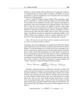
FIGURE 2.20 Change in instruction count for the programs hydro2d and li from the SPEC92 as compiler optimi-
zation levels vary. Level 0 is the same as unoptimized code. These experiments were perfomed on the MIPS compilers.
Level 1 includes local optimizations, code scheduling, and local register allocation. Level 2 includes global optimizations,
loop transformations (

software pipelining
), and global register allocation. Level 3 adds procedure integration.
li level 0
0% 20% 40% 60% 80% 100%
li level 1
li level 2
li level 3
hydro l 0
hydro l 1
hydro l 2
hydro l 3
100%
89%
75%
73%
100%
36%
26%
26%
Program and compiler
optimization level
FLOPs Loads-stores Integer ALUBranches/calls
Percent of unoptimized instructions executed
2.7 Crosscutting Issues: The Role of Compilers 95
How the Architect Can Help the Compiler Writer
Today, the complexity of a compiler does not come from translating simple state-
ments like A = B + C. Most programs are locally simple, and simple translations
work fine. Rather, complexity arises because programs are large and globally
complex in their interactions, and because the structure of compilers means that
decisions must be made about what code sequence is best one step at a time.

Compiler writers often are working under their own corollary of a basic prin-
ciple in architecture: Make the frequent cases fast and the rare case correct. That
is, if we know which cases are frequent and which are rare, and if generating
code for both is straightforward, then the quality of the code for the rare case may
not be very important—but it must be correct!
Some instruction set properties help the compiler writer. These properties
should not be thought of as hard and fast rules, but rather as guidelines that will
make it easier to write a compiler that will generate efficient and correct code.
1. Regularity;—Whenever it makes sense, the three primary components of an in-
struction set—the operations, the data types, and the addressing modes—
should be orthogonal. Two aspects of an architecture are said to be orthogonal
if they are independent. For example, the operations and addressing modes are
orthogonal if for every operation to which a certain addressing mode can be
applied, all addressing modes are applicable. This helps simplify code genera-
tion and is particularly important when the decision about what code to gener-
ate is split into two passes in the compiler. A good counterexample of this
property is restricting what registers can be used for a certain class of instruc-
tions. This can result in the compiler finding itself with lots of available regis-
ters, but none of the right kind!
2. Provide primitives, not solutions—Special features that “match” a language
construct are often unusable. Attempts to support high-level languages may
work only with one language, or do more or less than is required for a correct
and efficient implementation of the language. Some examples of how these at-
tempts have failed are given in section 2.9.
3. Simplify trade-offs among alternatives—One of the toughest jobs a compiler
writer has is figuring out what instruction sequence will be best for every seg-
ment of code that arises. In earlier days, instruction counts or total code size
might have been good metrics, but—as we saw in the last chapter—this is no
longer true. With caches and pipelining, the trade-offs have become very com-
plex. Anything the designer can do to help the compiler writer understand the

costs of alternative code sequences would help improve the code. One of the
most difficult instances of complex trade-offs occurs in a register-memory
architecture in deciding how many times a variable should be referenced be-
fore it is cheaper to load it into a register. This threshold is hard to compute
and, in fact, may vary among models of the same architecture.
96 Chapter 2 Instruction Set Principles and Examples
4. Provide instructions that bind the quantities known at compile time as con-
stants—A compiler writer hates the thought of the machine interpreting at
runtime a value that was known at compile time. Good counterexamples of
this principle include instructions that interpret values that were fixed at com-
pile time. For instance, the VAX procedure call instruction (calls) dynami-
cally interprets a mask saying what registers to save on a call, but the mask is
fixed at compile time. However, in some cases it may not be known by the
caller whether separate compilation was used.
Summary: The Role of Compilers
This section leads to several recommendations. First, we expect a new instruction
set architecture to have at least 16 general-purpose registers—not counting sepa-
rate registers for floating-point numbers—to simplify allocation of registers using
graph coloring. The advice on orthogonality suggests that all supported address-
ing modes apply to all instructions that transfer data. Finally, the last three pieces
of advice of the last subsection—provide primitives instead of solutions, simplify
trade-offs between alternatives, don’t bind constants at runtime—all suggest that
it is better to err on the side of simplicity. In other words, understand that less is
more in the design of an instruction set.
In many places throughout this book we will have occasion to refer to a comput-
er’s “machine language.” The machine we use is a mythical computer called
“MIX.” MIX is very much like nearly every computer in existence, except that it
is, perhaps, nicer … MIX is the world’s first polyunsaturated computer. Like most
machines, it has an identifying number—the 1009. This number was found by tak-
ing 16 actual computers which are very similar to MIX and on which MIX can be

easily simulated, then averaging their number with equal weight:

(360 + 650 + 709 + 7070 + U3 + SS80 + 1107 + 1604 + G20 + B220 + S2000
+ 920 + 601 + H800 + PDP-4 + II)/16

= 1009.
The same number may be obtained in a simpler way by taking Roman numerals.
Donald Knuth, The Art of Computer Programming, Volume I: Fundamental Algorithms
In this section we will describe a simple load-store architecture called DLX (pro-
nounced “Deluxe”). The authors believe DLX to be the world’s second polyun-
saturated computer—the average of a number of recent experimental and
commercial machines that are very similar in philosophy to DLX. Like Knuth,
2.8
Putting It All Together: The DLX Architecture
2.8 Putting It All Together: The DLX Architecture 97
we derived the name of our machine from an average expressed in Roman
numerals:
(AMD 29K, DECstation 3100, HP 850, IBM 801, Intel i860, MIPS M/120A,
MIPS M/1000, Motorola 88K, RISC I, SGI 4D/60, SPARCstation-1, Sun-4/110,
Sun-4/260) / 13 = 560 = DLX.
The instruction set architecture of DLX and its ancestors was based on obser-
vations similar to those covered in the last sections. (In section 2.11 we discuss
how and why these architectures became popular.) Reviewing our expectations
from each section:
■ Section 2.2—Use general-purpose registers with a load-store architecture.
■ Section 2.3—Support these addressing modes: displacement (with an address
offset size of 12 to 16 bits), immediate (size 8 to 16 bits), and register deferred.
■ Section 2.4—Support these simple instructions, since they will dominate the
number of instructions executed: load, store, add, subtract, move register-
register, and, shift, compare equal, compare not equal, branch (with a PC-rela-

tive address at least 8 bits long), jump, call, and return.
■ Section 2.5—Support these data sizes and types: 8-, 16-, and 32-bit integers and
64-bit IEEE 754 floating-point numbers.
■ Section 2.6—Use fixed instruction encoding if interested in performance and
use variable instruction encoding if interested in code size.
■ Section 2.7—Provide at least 16 general-purpose registers plus separate floating-
point registers, be sure all addressing modes apply to all data transfer instruc-
tions, and aim for a minimalist instruction set.
We introduce DLX by showing how it follows these recommendations. Like
most recent machines, DLX emphasizes
■ A simple load-store instruction set
■ Design for pipelining efficiency, including a fixed instruction set encoding
(discussed in Chapter 3)
■ Efficiency as a compiler target
DLX provides a good architectural model for study, not only because of the re-
cent popularity of this type of machine, but also because it is an easy architecture
to understand. We will use this architecture again in Chapters 3 and 4, and it
forms the basis for a number of exercises and programming projects.
98 Chapter 2 Instruction Set Principles and Examples
Registers for DLX
DLX has 32 32-bit general-purpose registers (GPRs), named R0, R1, …, R31.
Additionally, there is a set of floating-point registers (FPRs), which can be used
as 32 single-precision (32-bit) registers or as even-odd pairs holding double-
precision values. Thus, the 64-bit floating-point registers are named F0, F2, ,
F28, F30. Both single- and double-precision floating-point operations (32-bit and
64-bit) are provided.
The value of R0 is always 0. We shall see later how we can use this register to
synthesize a variety of useful operations from a simple instruction set.
A few special registers can be transferred to and from the integer registers. An
example is the floating-point status register, used to hold information about the

results of floating-point operations. There are also instructions for moving be-
tween a FPR and a GPR.
Data types for DLX
The data types are 8-bit bytes, 16-bit half words, and 32-bit words for integer data
and 32-bit single precision and 64-bit double precision for floating point. Half
words were added to the minimal set of recommended data types supported
because they are found in languages like C and popular in some programs, such as
the operating systems, concerned about size of data structures. They will also
become more popular as Unicode becomes more widely used. Single-precision
floating-point operands were added for similar reasons. (Remember the early
warning that you should measure many more programs before designing an
instruction set.)
The DLX operations work on 32-bit integers and 32- or 64-bit floating point.
Bytes and half words are loaded into registers with either zeros or the sign bit
replicated to fill the 32 bits of the registers. Once loaded, they are operated on
with the 32-bit integer operations.
Addressing modes for DLX data transfers
The only data addressing modes are immediate and displacement, both with 16-
bit fields. Register deferred is accomplished simply by placing 0 in the 16-bit dis-
placement field, and absolute addressing with a 16-bit field is accomplished by
using register 0 as the base register. This gives us four effective modes, although
only two are supported in the architecture.
DLX memory is byte addressable in Big Endian mode with a 32-bit address. As
it is a load-store architecture, all memory references are through loads or stores
between memory and either the GPRs or the FPRs. Supporting the data types
mentioned above, memory accesses involving the GPRs can be to a byte, to a half
word, or to a word. The FPRs may be loaded and stored with single-precision or
double-precision words (using a pair of registers for DP). All memory accesses
must be aligned.
2.8 Putting It All Together: The DLX Architecture 99

DLX Instruction Format
Since DLX has just two addressing modes, these can be encoded into the opcode.
Following the advice on making the machine easy to pipeline and decode, all in-
structions are 32 bits with a 6-bit primary opcode. Figure 2.21 shows the instruc-
tion layout. These formats are simple while providing 16-bit fields for
displacement addressing, immediate constants, or PC-relative branch addresses.
DLX Operations
DLX supports the list of simple operations recommended above plus a few oth-
ers. There are four broad classes of instructions: loads and stores, ALU opera-
tions, branches and jumps, and floating-point operations.
Any of the general-purpose or floating-point registers may be loaded or stored,
except that loading R0 has no effect. Single-precision floating-point numbers oc-
cupy a single floating-point register, while double-precision values occupy a pair.
Conversions between single and double precision must be done explicitly. The
floating-point format is IEEE 754 (see Appendix A). Figure 2.22 gives examples
FIGURE 2.21 Instruction layout for DLX. All instructions are encoded in one of three
types.
I-type instruction
rs1 rd Immediate
Encodes: Loads and stores of bytes, words, half words
All immediates (rd rs1 op immediate)
65 5 16
Conditional branch instructions (rs1 is register, rd unused)
Jump register, jump and link register
(rd = 0, rs1 = destination, immediate = 0)
R-type instruction
rs1 rs2
Register–register ALU operations: rd rs1 func rs2
Function encodes the data path operation: Add, Sub, . . .
Read/write special registers and moves

655 115
func
Opcode
J-type instruction
Offset added to PC
626
Jump and jump and link
Trap and return from exception
Opcode
Opcode rd
–‹
–‹
100 Chapter 2 Instruction Set Principles and Examples
of the load and store instructions. A complete list of the instructions appears in
Figure 2.25 (page 104). To understand these figures we need to introduce a few
additional extensions to our C description language:
■ A subscript is appended to the symbol ← whenever the length of the datum be-
ing transferred might not be clear. Thus, ←
n
means transfer an n-bit quantity.
We use x, y ← z to indicate that z should be transferred to x and y.
■ A subscript is used to indicate selection of a bit from a field. Bits are labeled
from the most-significant bit starting at 0. The subscript may be a single digit
(e.g., Regs[R4]
0
yields the sign bit of R4) or a subrange (e.g., Regs[R3]
24 31
yields the least-significant byte of R3).
■ The variable Mem, used as an array that stands for main memory, is indexed by
a byte address and may transfer any number of bytes.

■ A superscript is used to replicate a field (e.g., 0
24
yields a field of zeros of
length 24 bits).
■ The symbol ## is used to concatenate two fields and may appear on either side
of a data transfer.
Example instruction Instruction name Meaning
LW R1,30(R2) Load word Regs[R1]←
32
Mem[30+Regs[R2]]
LW R1,1000(R0) Load word Regs[R1]←
32
Mem[1000+0]
LB R1,40(R3) Load byte Regs[R1]←
32
(Mem[40+Regs[R3]]
0
)
24
##
Mem[40+Regs[R3]]
LBU R1,40(R3) Load byte unsigned Regs[R1]←
32
0
24
## Mem[40+Regs[R3]]
LH R1,40(R3) Load half word Regs[R1]←
32
(Mem[40+Regs[R3]]
0

)
16
##
Mem[40+Regs[R3]]##Mem[41+Regs[R3]]
LF F0,50(R3) Load float Regs[F0]←
32
Mem[50+Regs[R3]]
LD F0,50(R2) Load double Regs[F0]##Regs[F1]←
64
Mem[50+Regs[R2]]
SW R3,500(R4) Store word Mem[500+Regs[R4]]←
32
Regs[R3]
SF F0,40(R3) Store float Mem[40+Regs[R3]]←
32
Regs[F0]
SD F0,40(R3) Store double Mem[40+Regs[R3]]←
32
Regs[F0];
Mem[44+Regs[R3]]←
32
Regs[F1]
SH R3,502(R2) Store half Mem[502+Regs[R2]]←
16
Regs[R3]
16 31
SB R2,41(R3) Store byte Mem[41+Regs[R3]]←
8
Regs[R2]
24 31

FIGURE 2.22 The load and store instructions in DLX. All use a single addressing mode and require that the memory
value be aligned. Of course, both loads and stores are available for all the data types shown.
2.8 Putting It All Together: The DLX Architecture 101
A summary of the entire description language appears on the back inside
cover. As an example, assuming that R8 and R10 are 32-bit registers:
Regs[R10]
16 31
←
16
(Mem[Regs[R8]]
0
)
8

## Mem[Regs[R8]]
means that the byte at the memory location addressed by the contents of R8 is
sign-extended to form a 16-bit quantity that is stored into the lower half of R10.
(The upper half of R10 is unchanged.)
All ALU instructions are register-register instructions. The operations include
simple arithmetic and logical operations: add, subtract, AND, OR, XOR, and shifts.
Immediate forms of all these instructions, with a 16-bit sign-extended immediate,
are provided. The operation LHI (load high immediate) loads the top half of a
register, while setting the lower half to 0. This allows a full 32-bit constant to be
built in two instructions, or a data transfer using any constant 32-bit address in
one extra instruction.
As mentioned above, R0 is used to synthesize popular operations. Loading a
constant is simply an add immediate where one of the source operands is R0, and
a register-register move is simply an add where one of the sources is R0. (We
sometimes use the mnemonic LI, standing for load immediate, to represent the
former and the mnemonic MOV for the latter.)

There are also compare instructions, which compare two registers (=, ≠, <, >,
≤, ≥). If the condition is true, these instructions place a 1 in the destination regis-
ter (to represent true); otherwise they place the value 0. Because these operations
“set” a register, they are called set-equal, set-not-equal, set-less-than, and so on.
There are also immediate forms of these compares. Figure 2.23 gives some ex-
amples of the arithmetic/logical instructions.
Control is handled through a set of jumps and a set of branches. The four jump
instructions are differentiated by the two ways to specify the destination address
and by whether or not a link is made. Two jumps use a 26-bit signed offset added
Example instruction Instruction name Meaning
ADD R1,R2,R3 Add Regs[R1]←Regs[R2]+Regs[R3]
ADDI R1,R2,#3 Add immediate Regs[R1]←Regs[R2]+3
LHI R1,#42 Load high immediate
Regs[R1]←42##0
16
SLLI R1,R2,#5 Shift left logical
immediate
Regs[R1]←Regs[R2]<<5
SLT R1,R2,R3 Set less than if (Regs[R2]<Regs[R3])
Regs[R1]←1 else Regs[R1]←0
FIGURE 2.23 Examples of arithmetic/logical instructions on DLX, both with and without im-
mediates.
102 Chapter 2 Instruction Set Principles and Examples
to the program counter (of the instruction sequentially following the jump) to de-
termine the destination address; the other two jump instructions specify a register
that contains the destination address. There are two flavors of jumps: plain jump,
and jump and link (used for procedure calls). The latter places the return
address—the address of the next sequential instruction—in R31.
All branches are conditional. The branch condition is specified by the in-
struction, which may test the register source for zero or nonzero; the register may

contain a data value or the result of a compare. The branch target address is spec-
ified with a 16-bit signed offset that is added to the program counter, which is
pointing to the next sequential instruction. Figure 2.24 gives some typical branch
and jump instructions. There is also a branch to test the floating-point status reg-
ister for floating-point conditional branches, described below.
Floating-point instructions manipulate the floating-point registers and indicate
whether the operation to be performed is single or double precision. The opera-
tions
MOVF and MOVD copy a single-precision (MOVF) or double-precision (MOVD)
floating-point register to another register of the same type. The operations
MOVFP2I and MOVI2FP move data between a single floating-point register and an
integer register; moving a double-precision value to two integer registers requires
two instructions. Integer multiply and divide that work on 32-bit floating-point
registers are also provided, as are conversions from integer to floating point and
vice versa.
The floating-point operations are add, subtract, multiply, and divide; a suffix D
is used for double precision and a suffix F is used for single precision (e.g., ADDD,
ADDF, SUBD, SUBF, MULTD, MULTF, DIVD, DIVF). Floating-point compares set a
Example instruction Instruction name Meaning
J name Jump
PC←name; ((PC+4)–2
25
) ≤ name <
((PC+4)+2
25
)
JAL name Jump and link Regs[R31]←PC+4; PC←name;
((PC+4)–2
25
)

≤ name < ((PC+4)+2
25
)
JALR R2 Jump and link register Regs[R31]←PC+4; PC←Regs[R2]
JR R3 Jump register PC←Regs[R3]
BEQZ R4,name Branch equal zero if (Regs[R4]==0) PC←name;
((PC+4)–2
15
)

≤ name < ((PC+4)+2
15
)
BNEZ R4,name Branch not equal zero if (Regs[R4]!=0) PC←name;
((PC+4)–2
15
)

≤ name < ((PC+4)+2
15
)
FIGURE 2.24 Typical control-flow instructions in DLX. All control instructions, except jumps to an address in a register,
are PC-relative. If the register operand is R0, BEQZ will always branch, but the compiler will usually prefer to use a jump with
a longer offset over this “unconditional branch.”
2.8 Putting It All Together: The DLX Architecture 103
bit in the special floating-point status register that can be tested with a pair of
branches: BFPT and BFPF, branch floating-point true and branch floating-point
false.
One slightly unusual DLX characteristic is that it uses the floating-point unit

for integer multiplies and divides. As we shall see in Chapters 3 and 4, the control
for the slower floating-point operations is much more complicated than for inte-
ger addition and subtraction. Since the floating-point unit already handles float-
ing point multiply and divide, it is not much harder for it to perform the relatively
slow operations of integer multiply and divide. Hence DLX requires that oper-
ands to be multiplied or divided be placed in floating-point registers.
Figure 2.25 contains a list of all DLX operations and their meaning. To give
an idea which instructions are popular, Figure 2.26 shows the frequency of in-
structions and instruction classes for five SPECint92 programs and Figure 2.27
shows the same data for five SPECfp92 programs. To give a more intuitive feel-
ing, Figures 2.28 and 2.29 show the data graphically for all instructions that are
responsible on average for more than 1% of the instructions executed.
Effectiveness of DLX
It would seem that an architecture with simple instruction formats, simple ad-
dress modes, and simple operations would be slow, in part because it has to exe-
cute more instructions than more sophisticated designs. The performance
equation from the last chapter reminds us that execution time is a function of
more than just instruction count:
To see whether reduction in instruction count is offset by increases in CPI or
clock cycle time, we need to compare DLX to a sophisticated alternative.
One example of a sophisticated instruction set architecture is the VAX. In the
mid 1970s, when the VAX was designed, the prevailing philosophy was to create
instruction sets that were close to programming languages to simplify compilers.
For example, because programming languages had loops, instruction sets should
have loop instructions, not just simple conditional branches; they needed call in-
structions that saved registers, not just simple jump and links; they needed case
instructions, not just jump indirect; and so on. Following similar arguments, the
VAX provided a large set of addressing modes and made sure that all addressing
modes worked with all operations. Another prevailing philosophy was to mini-
mize code size. Recall that DRAMs have grown in capacity by a factor of four

every three years; thus in the mid 1970s DRAM chips contained less than 1/1000
the capacity of today’s DRAMs, so code space was also critical. Code space was
CPU

time Instruction

count CPI

×

Clock

cycle

time

×

=

104

Chapter 2 Instruction Set Principles and Examples

Instruction type/opcode Instruction meaning
Data transfers Move data between registers and memory, or between the integer and FP or special
registers; only memory address mode is 16-bit displacement + contents of a GPR

LB,LBU,SB

Load byte, load byte unsigned, store byte

LH,LHU,SH

Load half word, load half word unsigned, store half word

LW,SW

Load word, store word (to/from integer registers)

LF,LD,SF,SD

Load SP float, load DP float, store SP float, store DP float

MOVI2S, MOVS2I

Move from/to GPR to/from a special register

MOVF, MOVD

Copy one FP register or a DP pair to another register or pair

MOVFP2I,MOVI2FP

Move 32 bits from/to FP registers to/from integer registers

Arithmetic/logical Operations on integer or logical data in GPRs; signed arithmetic trap on overflow

ADD,ADDI,ADDU, ADDUI

Add, add immediate (all immediates are 16 bits); signed and unsigned

SUB,SUBI,SUBU, SUBUI

Subtract, subtract immediate; signed and unsigned

MULT,MULTU,DIV,DIVU

Multiply and divide, signed and unsigned; operands must be FP registers; all operations
take and yield 32-bit values

AND,ANDI

And, and immediate

OR,ORI,XOR,XORI

Or, or immediate, exclusive or, exclusive or immediate

LHI

Load high immediate—loads upper half of register with immediate

SLL, SRL, SRA, SLLI,
SRLI, SRAI

Shifts: both immediate (

S__I)

and variable form (

S__)

; shifts are shift left logical, right
logical, right arithmetic

S__,S__I

Set conditional: “__” may be

LT,GT,LE,GE,EQ,NE

Control Conditional branches and jumps; PC-relative or through register

BEQZ,BNEZ

Branch GPR equal/not equal to zero; 16-bit offset from PC+4

BFPT,BFPF

Test comparison bit in the FP status register and branch; 16-bit offset from PC+4

J, JR

Jumps: 26-bit offset from PC+4 (

J

) or target in register (

JR)
JAL, JALR Jump and link: save PC+4 in R31, target is PC-relative (JAL) or a register (JALR)
TRAP Transfer to operating system at a vectored address
RFE Return to user code from an exception; restore user mode
Floating point FP operations on DP and SP formats
ADDD,ADDF Add DP, SP numbers
SUBD,SUBF Subtract DP, SP numbers
MULTD,MULTF Multiply DP, SP floating point
DIVD,DIVF Divide DP, SP floating point
CVTF2D, CVTF2I,
CVTD2F, CVTD2I,
CVTI2F, CVTI2D
Convert instructions: CVTx2y converts from type x to type y, where x and y are I
(integer), D (double precision), or F (single precision). Both operands are FPRs.
__D,__F DP and SP compares: “__” = LT,GT,LE,GE,EQ,NE; sets bit in FP status register
FIGURE 2.25 Complete list of the instructions in DLX. The formats of these instructions are shown in Figure 2.21.
SP = single precision; DP = double precision. This list can also be found on the page preceding the back inside cover.
2.8 Putting It All Together: The DLX Architecture 105
de-emphasized in fixed-length instruction sets like DLX. For example, DLX ad-
dress fields always use 16 bits, even when the address is very small. In contrast,
the VAX allows instructions to be a variable number of bytes, so there is little
wasted space in address fields.
Designers of VAX machines later performed a quantitative comparison of
VAX and a DLX-like machine for implementations with comparable organiza-
tions. Their choices were the VAX 8700 and the MIPS M2000. The differing
Instruction compress eqntott espresso gcc (cc1) li
Integer
average
load 19.8% 30.6% 20.9% 22.8% 31.3% 26%

store 5.6% 0.6% 5.1% 14.3% 16.7% 9%
add 14.4% 8.5% 23.8% 14.6% 11.1% 14%
sub 1.8% 0.3% 0.5% 0%
mul 0.1% 0%
div 0%
compare 15.4% 26.5% 8.3% 12.4% 5.4% 14%
load imm 8.1% 1.5% 1.3% 6.8% 2.4% 4%
cond branch 17.4% 24.0% 15.0% 11.5% 14.6% 17%
jump 1.5% 0.9% 0.5% 1.3% 1.8% 1%
call 0.1% 0.5% 0.4% 1.1% 3.1% 1%
return, jmp ind 0.1% 0.5% 0.5% 1.5% 3.5% 1%
shift 6.5% 0.3% 7.0% 6.2% 0.7% 4%
and 2.1% 0.1% 9.4% 1.6% 2.1% 3%
or 6.0% 5.5% 4.8% 4.2% 6.2% 5%
other (xor, not) 1.0% 2.0% 0.5% 0.1% 1%
load FP 0%
store FP 0%
add FP 0%
sub FP 0%
mul FP 0%
div FP 0%
compare FP 0%
mov reg-reg FP 0%
other FP 0%
FIGURE 2.26 DLX instruction mix for five SPECint92 programs. Note that integer register-register move instructions
are included in the add instruction. Blank entries have the value 0.0%.
106 Chapter 2 Instruction Set Principles and Examples
goals for VAX and MIPS have led to very different architectures. The VAX goals,
simple compilers and code density, led to powerful addressing modes, powerful
instructions, efficient instruction encoding, and few registers. The MIPS goals

were high performance via pipelining, ease of hardware implementation, and
compatibility with highly optimizing compilers. These goals led to simple in-
structions, simple addressing modes, fixed-length instruction formats, and a large
number of registers.
Figure 2.30 shows the ratio of the number of instructions executed, the ratio of
CPIs, and the ratio of performance measured in clock cycles. Since the organizations
Instruction doduc ear hydro2d mdljdp2 su2cor FP average
load 1.4% 0.2% 0.1% 1.1% 3.6% 1%
store 1.3% 0.1% 0.1% 1.3% 1%
add 13.6% 13.6% 10.9% 4.7% 9.7% 11%
sub 0.3% 0.2% 0.7% 0%
mul 0%
div 0%
compare 3.2% 3.1% 1.2% 0.3% 1.3% 2%
load imm 2.2% 0.2% 2.2% 0.9% 1%
cond branch 8.0% 10.1% 11.7% 9.3% 2.6% 8%
jump 0.9% 0.4% 0.4% 0.1% 0%
call 0.5% 1.9% 0.3% 1%
return, jmp ind 0.6% 1.9% 0.3% 1%
shift 2.0% 0.2% 2.4% 1.3% 2.3% 2%
and 0.4% 0.1% 0.3% 0%
or 0.2% 0.1% 0.1% 0.1% 0%
other (xor, not) 0%
load FP 23.3% 19.8% 24.1% 25.9% 21.6% 23%
store FP 5.7% 11.4% 9.9% 10.0% 9.8% 9%
add FP 8.8% 7.3% 3.6% 8.5% 12.4% 8%
sub FP 3.8% 3.2% 7.9% 10.4% 5.9% 6%
mul FP 12.0% 9.6% 9.4% 13.9% 21.6% 13%
div FP 2.3% 1.6% 0.9% 0.7% 1%
compare FP 4.2% 6.4% 10.4% 9.3% 0.8% 6%

mov reg-reg FP 2.1% 1.8% 5.2% 0.9% 1.9% 2%
other FP 2.4% 8.4% 0.2% 0.2% 1.2% 2%
FIGURE 2.27 DLX instruction mix for five programs from SPECfp92. Note that integer register-register move instruc-
tions are included in the add instruction. Blank entries have the value 0.0%.
2.8 Putting It All Together: The DLX Architecture 107
FIGURE 2.28 Graphical display of instructions executed of the five programs from
SPECint92 in Figure 2.26. These instruction classes collectively are responsible on average
for 92% of instructions executed.
FIGURE 2.29 Graphical display of instructions executed of the five programs from
SPECfp92 in Figure 2.27. These instruction classes collectively are responsible on average
for just under 90% of instructions executed.
load int
conditional branch
add int
compare int
store int
or
shift
and
26%
16%
0% 5% 10% 15% 20% 25%
14%
13%
9%
5%
4%
3%
eqntott espresso gcc licompress
Total dynamic count

load FP
mul FP
add int
store FP
conditional branch
add FP
sub FP
compare FP
23%
13%
0% 5% 10% 15% 20% 25%
11%
9%
8%
8%
6%
6%
ear hydro2d mdljdp2 su2cordoduc
mov reg FP 2%
shift
2%
Total dynamic count
108 Chapter 2 Instruction Set Principles and Examples
were similar, clock cycle times were assumed to be the same. MIPS executes about
twice as many instructions as the VAX, while the CPI for the VAX is about six times
larger than that for the MIPS. Hence the MIPS M2000 has almost three times the
performance of the VAX 8700. Furthermore, much less hardware is needed to build
the MIPS CPU than the VAX CPU. This cost/performance gap is the reason the
company that used to make the VAX has dropped it and is now making a machine
similar to DLX.

Time and again architects have tripped on common, but erroneous, beliefs. In this
section we look at a few of them.
FIGURE 2.30 Ratio of MIPS M2000 to VAX 8700 in instructions executed and performance in clock cycles using
SPEC89 programs. On average, MIPS executes a little over twice as many instructions as the VAX, but the CPI for the VAX
is almost six times the MIPS CPI, yielding almost a threefold performance advantage. (Based on data from Bhandarkar and
Clark [1991].)
2.9
Fallacies and Pitfalls
0.0
0.5
1.0
1.5
2.0
2.5
3.0
3.5
4.0
li
eqntott
espresso
doduc
tomcatv
fpppp
nasa7
matrix
spice
Performance
ratio
Instructions
executed ratio

CPI ratio
SPEC 89 benchmarks
MIPS/VAX
2.9 Fallacies and Pitfalls 109
Pitfall: Designing a “high-level” instruction set feature specifically oriented
to supporting a high-level language structure.
Attempts to incorporate high-level language features in the instruction set have
led architects to provide powerful instructions with a wide range of flexibility.
But often these instructions do more work than is required in the frequent case, or
they don’t exactly match the requirements of the language. Many such efforts
have been aimed at eliminating what in the 1970s was called the semantic gap.
Although the idea is to supplement the instruction set with additions that bring
the hardware up to the level of the language, the additions can generate what
Wulf [1981] has called a semantic clash:
by giving too much semantic content to the instruction, the machine designer
made it possible to use the instruction only in limited contexts. [p. 43]
More often the instructions are simply overkill—they are too general for the
most frequent case, resulting in unneeded work and a slower instruction. Again,
the VAX CALLS is a good example. CALLS uses a callee-save strategy (the regis-
ters to be saved are specified by the callee) but the saving is done by the call in-
struction in the caller. The CALLS instruction begins with the arguments pushed
on the stack, and then takes the following steps:
1. Align the stack if needed.
2. Push the argument count on the stack.
3. Save the registers indicated by the procedure call mask on the stack (as men-
tioned in section 2.7). The mask is kept in the called procedure’s code—this
permits callee save to be done by the caller even with separate compilation.
4. Push the return address on the stack, then push the top and base of stack point-
ers for the activation record.
5. Clear the condition codes, which sets the trap enables to a known state.

6. Push a word for status information and a zero word on the stack.
7. Update the two stack pointers.
8. Branch to the first instruction of the procedure.
The vast majority of calls in real programs do not require this amount of over-
head. Most procedures know their argument counts, and a much faster linkage
convention can be established using registers to pass arguments rather than the
stack. Furthermore, the CALLS instruction forces two registers to be used for link-
age, while many languages require only one linkage register. Many attempts to
support procedure call and activation stack management have failed to be useful,
either because they do not match the language needs or because they are too
general and hence too expensive to use.