Báo cáo lâm nghiệp: "Variability and heterogeneity of humus forms at stand level: Comparison between pure beech and mixed beech-hornbeam forest" ppsx
Bạn đang xem bản rút gọn của tài liệu. Xem và tải ngay bản đầy đủ của tài liệu tại đây (683.81 KB, 12 trang )
177
Ann. For. Sci. 63 (2006) 177–188
© INRA, EDP Sciences, 2006
DOI: 10.1051/forest:2005110
Original article
Variability and heterogeneity of humus forms at stand level:
Comparison between pure beech and mixed beech-hornbeam forest
Michaël AUBERT*, Pierre MARGERIE, Aude ERNOULT, Thibaud DECAËNS, Fabrice BUREAU
Groupe de recherche ECODIV, UPRES-EA 1293, Faculté des Sciences et des Techniques, Université de Rouen,
76821 Mont-Saint-Aignan Cedex, France
(Received 17 January 2005; accepted 24 August 2005)
Abstract – We investigate the influence of tree canopy composition on humus form variability and heterogeneity by comparing a pure beech
stand and a mixed beech-hornbeam one (70% beech and 30% hornbeam). Macro-morphological humus form descriptors were recorded using
a spatially explicit sample design at stand level. Leaf litter composition and light intensity accounting for stand management as well as bulk
density for harvesting practices (soil compaction) were also recorded. A multiple correspondence analysis (MCA) and geostatistics were used
to assess humus form variability and heterogeneity, as well as the spatial correlation between stand characteristics and humus forms. Humus
form variability and activity were greater under the mixed stand than under the pure one. Geostatistics revealed that humus form patchiness was
greater under the mixed stand than under the pure one and the improvement in decomposition processes seemed to be confined to spatial
distribution of hornbeam litterfall. From a practical viewpoint, these results could provide ideas on the way of mixing tree species at stand level.
We assume that with a given percentage of mull-forming tree species, a dispersed tree mixture provides a more extensive improvement than a
clumped mixture.
humus form / pure stand / mixed stand / geostatistics / spatial pattern / heterogeneity / Fagus sylvatica / Carpinus betulus
Résumé – Variabilité et hétérogénéité des formes d’humus à l’échelle du peuplement : comparaison entre peuplement pur de hêtre et
forêt mélangée hêtre-charme. Nous avons étudié l’influence de la composition d’un peuplement sur la variabilité qualitative et l’hétérogénéité
spatiale des formes d’humus en comparant un peuplement pur de hêtre et un peuplement mélangé (70 % hêtre – 30 % charme). Les
caractéristiques macro-morphologiques des formes d’humus ainsi que la composition spécifique de la litière, l’éclairement relatif sous le
peuplement et la densité apparente du sol ont été mesurées à l’aide d’un échantillonnage spatialement explicite. Une analyse des
correspondances multiples (ACM) couplée à des géostatistiques a été utilisée pour caractériser la variabilité et l’hétérogénéité des formes
d’humus ainsi que leur corrélation spatiale avec les caractéristiques de peuplement. La variabilité, l’hétérogénéité et l’activité des formes
d’humus sont plus fortes sous peuplement mixte. Sous ce peuplement, l’amélioration de l’activité des formes d’humus est liée à la distribution
spatiale des retombées de feuilles de charme. Ces résultats semblent indiquer que, pour un pourcentage donné d’une espèce ligneuse à litière
améliorante, un mélange d’arbre par pied a un meilleur impact sur les formes d’humus qu’un mélange par bouquet.
forme d’humus / peuplement pur / peuplement mélangé / géostatistiques / patrons spatiaux / hétérogénéité / Fagus sylvatica / Carpinus betulus
1. INTRODUCTION
Humus form is defined as the group of organic and organic-
enriched mineral horizons at the soil surface [33, 55]. Humus
form descriptions are currently based on morphological prop-
erties. Moreover, in the French classification [1, 17], it is the
entire macro-morphological features of the “épisolum humifère”
(i.e. humic epipedon according to [55]), which defines humus
forms consisting of the O and A horizons and their vertical
sequence. The vertical organisation of these constitutive hori-
zons is considered to be a great integrator of topsoil biological
activity [32, 34], which conditions the rate of decomposition
processes. Its importance for the productivity of terrestrial eco-
systems, such as forests, has largely been recognized [33].
Thus, the development of silvicultural practices promoting top-
soil mineralization has become a necessity for sustainable sil-
viculture [49].
There are many factors influencing humus form character-
istics, acting at various spatial and time scales such as topog-
raphy [28], parent material [48] and stand dynamics [3, 10, 13,
47] at a coarse scale, and microbial communities [53] or root
activity [45] at a fine scale. At stand level, canopy composition
and structure may influence humus forms. Concerning the
structure, the opening of canopy due to tree partial removal,
leading to more light reaching the soil, is thought to increase
organic matter decomposition [25] and thus to modify humus
form characteristics. Tree species composition and the position
of trees has also a strong influence on the organic layer prop-
erties [12, 43]. The chemical composition of leaves differs con-
siderably between tree species and affects litter decomposition
rate and humus quality [44]. It has been recognized for a long
time that the presence of mull-forming tree species within a
stand dominated by moder or mor-forming species provides a
* Corresponding author:
Article published by EDP Sciences and available at or />178 M. Aubert et al.
positive impact on organic layer properties [15, 20, 31, 46].
Although these studies underlined the better quality of humus
form in the presence of mull-forming species, the spatial pattern
of this improvement was not described. The question of the
existence and strength of spatial correlations between stand
composition and recorded variations in humus form properties
remains. Is this improvement localised near mull-forming spe-
cies or does it spread throughout the stand? Answering this
question could provide practical background for forest manag-
ers on whether to mix tree species in a dispersed or clumped
mixture.
In the present paper, we compare humus form variability and
heterogeneity in a pure beech stand (Fagus sylvatica L.) and a
mixed beech-hornbeam (Carpinus betulus L.) stand. Macro-
morphological humus form descriptors (including pH and
organic C and N) were recorded using a spatially explicit sam-
ple design at stand level. Variability, i.e. changes in the values
of a given property [37], was assessed by multivariate analysis.
Heterogeneity, i.e. spatial structure of variability [62], was
quantified using geostatistics [28]. Moreover, three variables
supposed to influence humus form features were recorded: leaf lit-
ter composition, light intensity accounting for stand manage-
ment as well as bulk density for harvesting practices (soil com-
paction). The aim of this study was to test four hypotheses:
(1) Variability of humus form is greater under a mixed
stand than under a pure stand,
(2) Humus form is on average more active under a mixed
than under a pure stand,
(3) Humus form is more heterogeneous under a mixed can-
opy than under a pure one,
(4) The improving effect of hornbeam is limited to the
hornbeam litterfall distribution rather than spreading
throughout the stand.
2. MATERIALS AND METHODS
2.1. Definition and nomenclature of humus forms
According to [1], soil horizons containing organic matter can be
divided in: (i) holorganic horizons (O horizons) almost without min-
eral material and (ii) organo-mineral horizon (A horizon) below. O
horizons can be divided into three types according to the degree of litter
transformation [34]:
• OL (Oi in USDA nomenclature) consisting of almost unmodified
leaf and woody fragments. This horizon can be divided into:
(i) OLn consisting of litter less than one year old without obvious
decomposition; and (ii) OLv consisting of litter more than one
year old with coloration changes, cohesion and hardness mainly
due to fungal activity.
• OF (Oe in USDA nomenclature): consisting of a mixture of
coarse plant fragments with fine organic matter (FOM) resulting
from faecal pellets accumulation. Depending on the percentage
of FOM, this horizon can de divided into OFr (less than 30%
FOM) and OFm (30–70% FOM). As earthworm activity is redu-
ced, leaf transformation is attributed to the activity of soil epigeic
fauna and fungi.
• OH (Oa in USDA nomenclature): more than 70% FOM corres-
ponding to accumulation of faecal pellets and fine plant frag-
ments. It can be divided into OHr with 70 to 90% FOM and OHf
with 90 to 100%.
“Humus forms” is the macro-morphological description of the
humic epipedon (the French “épisolum humifère”) i.e. the vertical
sequence of its constitutive horizons. It results from active processes
in the different layers [18]. According to Brêthes [16], the main humus
forms occurring in beech forest of Upper-Normandy located on very
acidic and oligosaturated Luvisols are:
• Oligomull (usual horizon sequence: OL, (OF)/structured A);
• Dysmull (usual horizon sequence: OL, OF/structured A);
• Hemimoder (usual horizon sequence: OL, OF/unstructured A);
• Eumoder (usual horizon sequence: OL, OF, OH (thin)/unstruc-
tured A);
• Dysmoder (usual horizon sequence: OL, OF, OH (thick)/uns-
tructured A).
Correspondence with Green et al. classification [33] is as follows:
Oligomull = Hemimor, Dysmull = Leptomoder and Hemi-, Eu- and
Dysmoder = Leptomoder or Mormoder.
2.2. Sites description
The two stands are located in Upper-Normandy (northern France).
The pure beech stand belongs to the state forest of Eawy (01° 18’ E;
49° 44’ N; 205 m a.s.l.). The mixed beech-hornbeam one is located in
the state forest of Lyons (01° 37’ E; 49° 26’ N; 200 m a.s.l.). The mean
annual rainfall and temperature are 800 mm and 10 °C respectively.
Stand choice was guided so that differences in humus form varia-
bility and heterogeneity could be only due to stand characteristics
(stand composition and organisation) and not to site differences (cli-
mate, soil and management). Thus, stands were chosen with the same
vegetation succession stage i.e. a mature stand with a closed canopy
[2] characterised by: (i) ecological similarity of plant communities and
(ii) a low rate of litter incorporation [3]. According to phytosociolog-
ical classifications, both belonged to the Endymio-Fagetum [7]. Trees
were mapped and the breast height (1.3 m) diameters were measured
within the area of the sampling design (1 ha). The similarity of stand
structures was checked (see Tab. I). Both stands are situated in a top-
ographically flat area. They were characterised by the same parent
materials: more than 80 cm of loess (lamellated silts) resting on the
same type of clay with flints [38, 39]. Two soil profiles were described
for each stand thanks to two pedological pits located at two opposite
angles of the sampling grid. Physico-chemical analyses were performed
on the horizons of one soil profile for each stand (see appendix).
Table I. Stands description. Percent of beech, hornbeam, sessile oak
and holly represent the number of stems of these species as a per-
centage of the total number of stems. Values presented in parenthesis
represent the standard error. Mean RI (Relative Irradiance) is the
mean value of the 121-recorded measures on the sampling grid.
Pure stand Mixed stand
Age (years) 116 114
Last thinning operation 1995 1998
Number of tree (ha
–1
) 178 179
DBH (cm) 41.7 (17.8) 40.94 (13.62)
Basal area (m
2
.ha
–1
) 28.71 26.14
Percent of beech 94.38% 67.04%
Percent of hornbeam 0% 30.73%
Percent of sessile oak 5.06% 2.23%
Percent of holly 0.56% 0%
Mean RI 5.18 (0.78) 4.77 (0.61)
Variability and heterogeneity of humus form 179
The studied stands had grown on a very acid, low redox, oligosaturated
Luvisol according to the [1], equivalent to an endogleyic dystric Luvisol
in the World Reference Base [29].
2.3. Data collection
For both stands, the spatial pattern of humus form was investigated
using 121 points regularly distributed on a 10 m-mesh square grid (100
× 100 m) during winter 2000–2001. At each point, (i) 15 macro-mor-
phological variables were recorded and (ii) A horizon and the five cen-
timetres below, were sampled to estimate pH
H2O
, organic carbon and
total nitrogen. pH
H2O
was estimated according to Baize method [5]
i.e. on a 1:2.5 soil/liquid mixture using distilled water. Organic C and
total N were measured by gas chromatography with a CHN pyrolysis
micro-analyser. The C-N ratio was calculated for the A horizon.
twenty variables were recorded at each point of the sample grid for
both stands (Tab. II).
Three variables, which are likely to influence the spatial pattern of
humus form, were also recorded at each point: (i) Leaf litter compo-
sition [44], (ii) light intensity below canopy [13] and (iii) the impact
of harvesting methods on stand soil [6]. The OLn horizon was sampled
in the field and leaves were hand sorted in the laboratory to assess the
species composition of leaves expressed as percentage of OLn dry
weight. The light intensity below the canopy was estimated in July
2001 at each grid node by the means of the relative irradiance (RI) at
one metre above the soil, which is the light intensity under canopy/
light intensity outside the canopy, expressed as a percentage. The
impact of harvesting methods was assessed by estimating soil com-
paction [40]. This was measured by the bulk density (BD) [5]. Soil
cores (100 cm
3
) of the first 5 cm of the upper mineral soil were taken
at each node and dried at 105 °C for 3 days.
The presence near sampling points of tree trunks within 1.5 m, of
former windfalls, vehicle tracks, heaps of residual branches and
stumps were also recorded.
2.4. Statistical analysis
To assess how humus form variability and heterogeneity is affected
by the presence of hornbeam within a beech-dominated stand, multi-
variate and geostatistical analyses were used. First, a multiple corre-
spondence analysis (MCA) was computed to (i) extract the main
Table II. List of qualitative variables and their modalities used for humiferous episolum description.
Variables Modalities
OLv state 1) Absent 2) Present – discontinuous 3) Present – continuous
OFr state 1) Absent 2) Present – discontinuous 3) Present – continuous
OFm state 1) Absent 2) Present – discontinuous 3) Present – continuous
OHr state 1) Absent 2) Present – discontinuous 3) Present – continuous
A state 1) Absent 2) Present – discontinuous 3) Present – continuous
OLn thickness* 1) 0–1 cm 2) 1–3 cm 3) 3–6 cm
OLv thickness* 1) 0–0.5 cm 2) 0.5–1.5 cm 3) 1.5–3 cm
OFr thickness* 1) 0–0.5 cm 2) 0.5–1.5 cm 3) 1.5–2.5 cm
OFm thickness* 1) 0–0.5 cm 2) 0.5–1.5 cm 3) 1.5–3.5 cm
OHr thickness* 1) 0–0.2 cm 2) 0.2–0.6 cm 3) 0.6–1 cm
4) 1–2.1 cm
A thickness* 1) 0–0.5 cm 2) 0.5–1 cm 3) 1–2 cm
4) 2–6 cm
OHr/A transition 1) Sharp 2) Quite sharp 3) Progressive
A aggregate size 1) < 2 mm 2) 2–5 mm
A structure rank 1) Without aggregate 2) Slightly aggregated 3) Moderately aggregated
4) Strongly aggregated
A/E transition 1) > 8 cm 2) 4–8 cm 3) 2–4 cm
4) < 2 cm 5) Very sharp
A pH
H20
* 1) < 3.6 2) 3.6–4 3) > 4
A C-N ratio* 1) 8–15 2) 15–25 3) > 25
5 cm pH
H20
* 1) 3.5–4 2) 4–5.5
5 cm organic C* 1) < 2% 2) 2–4% 3) > 4%
5 cm total N* 1) < 0.05% 2) 0.05–0.1% 3) > 0.1%
* Indicates variables that were recorded as quantitative variables on the field and then converted into qualitative variables to perform the multiple cor-
respondence analysis. Division into modalities was made from a close examination of information gathered from very large published expert
knowledge [14, 17, 18, 32, 33, 34].
BD g.cm
–3
()
Core dry weight
Core volume
=
180 M. Aubert et al.
sources of variance in the data set and (ii) provide quantitative varia-
bles for geostatistical analysis. Secondarily, geostatistics (semi-vari-
ance analysis and the kriging procedure) were used to assess the spatial
structure of humus forms and produce maps. Cross-variance analysis
was performed between (i) sample scores along the main axes of the
MCA and (ii) variables (leaf litter composition, light intensity, soil
bulk density) supposed to influence humus forms and exhibiting struc-
tural variance. This was performed in order to account for spatial cor-
relation between humus forms and these variables.
2.4.1. Multiple correspondence analysis
MCA can be considered as a normalized principal component anal-
ysis (PCA) for categorical data [58]. Study sites were analysed
together in a data matrix of 242 records × 20 variables (64 variable
classes) (Tab. II). In order to help in interpreting MCA, the presence
(near sampling points) of tree trunks, former windfalls, vehicle tracks,
heaps of residual branches and stumps were projected as supplemen-
tary individuals in the subspaces defined by the main factors of vari-
ance underlined by the MCA.
A within inertia analysis was computed in order to extract the total
variance for each site in the MCA. Within-class inertia represents the
sum of the variance of each record forming a given class. Within a sam-
ple area, the greater the class variance is, the greater the spatial vari-
ability [62]. MCA and within-class inertia were computed with ADE
software [59].
2.4.2. Geostatistics
Geostatistics were used to quantify spatial patterns of soil biotic or
abiotic properties [28]. The method is based on the assumption that
points situated closed to one other in space share more similarities than
those farther apart [19]. In practice, geostatistical analysis is a two-
step procedure [43]:
First, the spatial structure of a given variable is estimated using
semi-variance analysis and described by a suitable model [52]. The
semi-variance γ for each specific distance interval h is calculated by:
where m(h) is the number of data point pairs separated by a particular
lag vector h (defined by both distance and direction); Z(x
i
) the meas-
ured value of the variable Z at point x
i
and Z(x
i
+ h) the sampled value
at a distance h [61]. The graph plotting γ and the distance between sam-
ples is called semi-variogram. Then, a theoretical model is fitted to the
semi-variogram calculated from sampled values [51]. Two main
model families exist: unbounded models where semi-variance appears
to be infinite and bounded models (more common) where γ reaches
a maximum for a given lag distance [61]. In this case, the maximum
semi-variance is called the “sill” and the distance at which the sill is
reached, is called the “range”. At lag 0, the intercept is called “nugget
variance” (C
0
). C
0
may have two origins: measurement errors and var-
iations at a smaller scale than that of the sampling design [52] i.e. 10 m
in our study. The proportion of the total variance that can be attributed
to the spatial autocorrelation is called the structural variance (C) and
is the difference between sill and nugget variance. C/[C + C
0
] ratio is
used to assess indicative values of the structural variance [11, 42, 43].
When it reaches 1, the whole sample variance is spatially dependent.
When it approaches 0, spatial dependence is low and factors accounting
for nugget variance are preponderant. To evaluate the goodness of a
model, a cross-validation procedure was used, which involves com-
paring kriged estimates and their variance [61]. The procedure is per-
formed by removing each data point in the data set and using remaining
data to predict it [36]. Three diagnostic statistics are calculated: (a) the
mean error (ME) which should ideally be 0; (b) the mean squared error
(MSE) which should approach 0 and (c) the mean squared deviation
ratio (MSDR) which should be 1.
where is kriging variance, Z(x
i
) is the observed value and
is the predicted value from cross-validation [36, 61].
The second step of a geostatistical analysis is the kriging procedure.
The aim of kriging is to estimate values of a given variable at unsam-
pled points using semi-variogram parameters [19, 28]. In this study,
we used ordinary kriging, which estimates the value Z of a variable at
a point x
0
using the formulae:
where λ
i
is a weight applied to each of the i neighbouring samples Z(x
i
)
[61]. λ
i
are derived from a set of equations determined by the vario-
gram model
parameters [51].
A cross semi-variance analysis was used to assess the spatial cor-
relation between two variables. This could reasonably be performed
between two variables exhibiting almost the same autocorrelation
range [61]. Two variables are cross-correlated when the values of one
at given places are correlated with the values of the other variable [51].
Spatial interdependence between two variables u and v is estimated
by the cross semi-variance :
where m(h) is the number of pairs of data points separated by a par-
ticular lag vector h, z(x
i
) the measured value of the variable Z at point
x
i
and z(x
i
+ h) the sampled value at a distance h. The graph plotting
the cross semi-variance against the distance h is called the cross-var-
iogram. Cross semi-variance is positive when the two variables are
positively correlated and negative in the opposite case . The cross
semi-variogram shows the same features as the semi-variogram [52].
Geostatistical analyses were performed on MCA record scores
(three first axes), stand characteristics (percent of hornbeam litter in
OLn and relative irradiance) and bulk density of soil (characteristic of
harvesting impact). Prior to this, a normality test was performed on the
variables using Statistix software [56]. If necessary, logarithmic trans-
formation was applied. Geostatistical analyses were performed using
Arcinfo 8.1, module Arcview, Geostatistical Analyst extension [27].
3. RESULTS
3.1. Variability
The total inertia of the performed MCA was 2.08. The first
three axes explained 18% of the total variance observed in quali-
tative variables accounting for humus forms description (Fig. 1).
γ h()
1
2mh()
Zx
i
() Zx
i
h+()–[]
2
i1=
mh()
∑
=
ME
1
N
Zx
i
() Zx
i
()–[]
i 1=
N
∑
=
MSE
1
N
Zx
i
() Zx
i
()–[]
2
i 1=
N
∑
=
MSDR
1
N
Zx
i
() Zx
i
()–[]
α
2
x
i
()
2
i 1=
N
∑
=
α
2
x
i
()
Zx
i
()
Zx
0
() λ
i
Zx
i
()
i 1=
n
∑
=
γ
uv
h(
)
γ
1
2mh()
z
u
x
i
() z
u
x
i
()–[]z
v
x
i
() z
v
x
i
h+()–[]
i1=
mh()
∑
=
Variability and heterogeneity of humus form 181
Sample clouds on the ordination diagram were represented by
ellipsoids containing 95% of points. The mixed stand (MS)
ellipsoid was more elongated on axes 1 and 2 than that of the
pure stand (PS). It was the opposite on axis 3. This indicated
that the range of sample variability within stands was greatest
for the mixed stand on axes 1 and 2 and for the pure stand on
axis 3. This is confirmed on the whole of MCA by the within
inertia analysis. The sum of the variance was 1.88 for PS
records and 2.18 for MS ones.
For each axis, only the most explicative variables were repre-
sented in the modalities ordination diagram of variable classes
(Fig. 2) depending on their correlation ratio (Tab. III). Axis 1
of the MCA accounted for 7.1% of the total inertia. The ordi-
nation of variable classes distinguished between (i) samples
characterised by a thick and continuous OFr and a thick A hori-
zon which was either strongly aggregated or not (negative part
of axis); and (ii) samples with a thick and continuous OHr and
a thin A horizon with weak aggregate size (positive part of the
axis). This axis clearly opposed dysmull and hemimoder in the
negative part from eumoder and dysmoder humus forms in the
positive part. According to the coordinates of the centre of grav-
ity of the ellipsoid on axis 1, the mixed stand tended towards
the more active humus forms while the pure stand tended
toward the less active ones (Fig. 1).
Axis 2 accounted for 5.8% of the total inertia. It separated
samples characterised by: (i) thick OL and OF horizons, a low
pH
H20
at 5 cm and a high percentage of organic carbon at 5 cm
(negative part); from (ii) samples with a thin OL and OF, a high
pH
H20
at 5 cm and low percentage of organic carbon at 5 cm
(positive part). The first category was mainly composed of sam-
ples recorded near tree trunks, stump or heaps of residual
branches and the second one of samples recorded near vehicle
Figure 1. Results of the Multiple Correspondence Analysis (MCA): (a) eigenvalues diagram; (b) sample ordination in the plan defined by axes
1 and 2 of the MCA; pure beech stand samples are shown by white squares and mixed stand ones by black points; for pure and mixed stands,
the centres of gravity of ellipsoids are equal to the mean of the sample coordinates; PS = pure beech stand; MS = mixed beech-hornbeam stand;
(c) projection as supplementary variables on the factorial plan 1–2 of the proximity of tree trunks to the sampling points (1), ancient windfalls
(2) vehicle tracks (3), heaps of residual branches (4), stumps (5) and without any special feature (6); (d) ordination of the samples in the plan
defined by axes 1 and 3.
182 M. Aubert et al.
tracks (see Fig. 1c). The macro-morphological characteristics
expressed the accumulation of organic matter (negative part)
and topsoil disturbances by harvesting practices (positive part).
Axis 3 accounted for 5.1% of the total inertia. It distin-
guished between: (i) samples with a thick and continuous OLv,
a discontinuous but thick OFr and an absent OHr (negative
part); and (ii) samples characterised by an absent OLv, a con-
tinuous but moderately thick OFr and a thick and continuous
OHr. This was interpreted as contrasting between humus forms
with a preponderant fungi activity and those in which soil
arthropod activity dominates.
3.2. Heterogeneity
Semi-variance analysis performed on MCA sample scores
and explicative variables showed that there was a great range
of variation in the degree of spatial dependence. The three dia-
gnostics of cross-validation (Tab. IV) validated the semi-vari-
ogram models for all variables except relative irradiance in
mixed stands (MSE = 16.605 and MSDR = 1.669).
The proportion of variance accounted for by the spatial
structure (Tab. IV) of humus form was on the whole low (rang-
ing from 0 to 21.93% of total variance) except for MS scores
on axis 1 (43.19%). The great resulting nugget effect indicated
that some spatial pattern might occur at smaller scale than that
of the sampling design. Nevertheless, MS scores on axis 1 had
Table III. Correlation coefficients between qualitative variables and
the first third axes of the MCA.
Variables r axis 1 r axis 2 r axis 3
OLv state 6 18.1 37.6
OFr state 30.5 11 32
OFm state. 2.1 13.1 14.5
OHr state. 42.1 4.9 18.4
A state 3.5 1.5 2
OLn thickness 13.2 35 1.3
OLv thickness 0.7 18.8 32.1
OFr thickness 35.4 20.5 31
OFm thickness 4.4 24.2 0.4
OHr thickness 41.7 7.5 22.3
A thickness 39.4 0.6 3.2
OHr/A tr. 8.2 1.3 0.7
A aggregate size. 18.7 6.8 4.7
A structure rank. 20 3.3 2.9
A/E transition 3.5 11.2 2.3
A pH
H2O
3.1 14.6 4.8
A C-N ratio 0.4 0.2 0.4
5 cm pH
H2O
6.4 23.2 0.6
5 cm organic C 11.3 19.2 1.7
5 cm total N 5.5 8.6 1.6
Figure 2. Ordination of variable classes (Tab. I) of
qualitative variables accounting for humus form
description; only the variables exhibiting the
highest correlation ratios with the three first MCA
axes are represented (see Tab. III).
Variability and heterogeneity of humus form 183
a greater structural variance than that of PS. The score autocor-
relation ranges were respectively 69.5 for MS and 91 for PS.
Kriging maps (Figs. 3 and 4) illustrated the stronger patchiness
of MS on axis 1 than that of PS.
With the exception of bulk density within MS, explicative
variables showed a higher structural variance than humus form.
Nevertheless, except for the percentage of hornbeam litter (HL)
within MS (85.46% of structural variance), there was a large
nugget effect. The HL autocorrelation range was about 65.5 m.
HL and MS scores on axis 1 were the variables exhibiting the
greatest structural variance. Moreover, their autocorrelation
ranges were very similar. Cross-semivariance analysis between
them revealed a negative co-regionalization for a distance of
less than 64 m (Fig. 5). The cross-validation procedure vali-
dated the fitted model. This meant that eumoder and dysmoder
humus forms were spatially correlated with a low percentage
of hornbeam litter in the OLn horizon. Cross-semivariance
analysis was performed between all other variables for each
stand but the resulting cross-semivariograms did not provide
significant results.
4. DISCUSSION
4.1. Humus forms variability
In the slightly desaturated loamy soil context of the North-
western France, multiple correspondence analysis interpreta-
tion showed that humus forms occurring within both stands
ranged from dysmull to dysmoder i.e. belonged to low-activity
humus forms [35]. The range of variation in humus forms was
greater under the mixed stand than under the pure one. This
result is in accordance with the first hypothesis. The presence
of hornbeam within the mixed stand seems to turn humus forms
toward the dysmull pole. This result supports hypothesis 2, that
humus form is more active in the mixed than in the pure stand.
This higher decomposition rate is beneficial for nutrient avail-
ability, tree growth and long-term site productivity [49, 60].
Nevertheless, Bernier [9] reported that humus profiles sampled
in comparable spruce stands in terms of tree age, showed only
slight functional differences. Moreover in coniferous forests in
the French Alps, Michalet et al. [41] found a discrepancy
between the very low biological activity of dysmull and its sta-
tus as mull in the French morphological classification [17].
Thus, as our differences between pure and mixed stands are
based on a macro-morphological description of humus forms,
they do not allow us to make any conclusions on functional dif-
ferences. The better quality of humus form within the mixed
stand may be the consequence of (i) the faster disappearance
of hornbeam leaves (due to their better quality than beech
leaves) and/or (ii) a greater biological activity under the mixed
stand than under the pure stand. The preponderant fungi activity
under the mixed stand (interpretation of MCA axis 3) tends to
confirm the second explanation. Nevertheless, further investi-
gations should be performed to search for a relation of cause
and effect between hornbeam litter quality and biological acti-
vity. According to Toutain [60], in the absence of anecic earth-
worms (which is the case for the studied sites [4]), white rot
fungi are the primary metabolizers of leaf brown pigments and
their rapid degradation may account for the formation of mull.
Tree trunks are recognized as having a strong influence on
humus form resulting in (i) an increase of organic layer thick-
ness and (ii) a decrease of A horizon pH [8, 23]. With regard
to the ordination of “stumps” within the factorial plan 1-2 of
the MCA, this influence seems to endure after tree felling.
Heaps of residual branches also represent a factor of organic
matter accumulation. Nevertheless, regarding its ordination
along the MCA axis 1 (Fig. 1c), this factor does not seem to
turn humus forms toward the dysmoder pole like the proximity
of tree trunk. Vehicle tracks, removing litter and exposing the
mineral horizons also have a strong influence on humus forms
characteristics [6, 22]. By revealing all these factors as second
Table IV. Semi-variogram model parameters for MCA samples scores and stand characteristics.
Stands Variables Model Nugget
(C0)
Sill
(C+C0)
C/C+C0
(× 100)
Range
(m)
Neighbourhood ME MSE MSDR
Pure Score axis 1 Exp 0.107 0.12 10.83 90.77 20 0.004 0.142 1.067
Score axis 2 Sph 0.075 0.085 11.76 22.14 5 –0.003 0.09 0.991
Score axis 3 Exp 0.115 0.115 0 20 –0.006 0.117 0.997
RI Sph 31.242 49.494 36.85 49.62 20 0.016 0.106 0.998
BD Exp 0.006 0.009 24.44 32.16 8 0.001 0.011 0.997
Mixed Score axis 1 Exp 0.081 0.141 43.19 69.64 20 0.004 0.113 1.004
Score axis 2 Exp 0.121 0.155 21.93 65.88 20 0.004 0.142 0.992
Score axis 3 Exp 0.079 0.087 8.04 76.64 20 –0.007 0.087 1.016
RI Exp 0.408 0.572 28.67 65.88 20 –0.078 16.605 1.669
BD Exp 0.00834 0.00863 3.36 88.60 20 0.001 0.011 1.008
%HL Sph 0.041 0.282 85.46 65.62 20 0.00008 0.088 1.002
Exp model: Exponential model; Sph model: Spherical model; RI: Relative irradiance; BD: Bulk density; %HL: Percent of hornbeam litter in OLn;
ME: Cross validation Mean Error; MSE: Cross validation mean squared error; MDSR: Cross validation mean squared deviation ratio.
184 M. Aubert et al.
Figure 3. Kriged maps of mixed beech-hornbeam stand: (a) MCA sample scores on axis 1; (b) sample scores on axis 2; (c) sample scores on
axis 3; (d) stand map; circles = beech; squares = hornbeam; triangles = oak; the size of circles, squares and triangles is proportional to trunks
diameter; (e) kriged map of relative irradiance; (f) kriged map of bulk density and (g) kriged map of the percent of hornbeam litter in OLn.
Variability and heterogeneity of humus form 185
order determinants, MCA indicates that, at stand level, harves-
ting practices have a strong impact on humus form.
4.2. Humus form spatial patterns
The aim of the study was to determine the influence of the
canopy composition patchiness on humus form. Geostatistical
analysis performed at our scale of investigation revealed that
the heterogeneity of humus forms, i.e. spatial structure of vari-
ability [62], is greater under the mixed stand than under the pure
one. As stand choice was guided so that differences in humus
form heterogeneity could be only due to stand characteristics,
this result supports our hypothesis 3.
Geostatistics performed at stand level revealed a strong nug-
get effect for most variables except MS scores on axis 1 and
the percentage of hornbeam leaves in OLn. This suggests that
spatial variations occurred at a distance smaller than our sam-
pling interval. In the forest ecosystems of British Columbia,
Qian and Klinka [50] reported that the spatial pattern of humus
Figure 4. Kriged maps of pure
beech stand: (a) MCA sample
scores on axis 1; (b) samples sco-
res on axis 2; (c) samples scores
on axis 3; (d) stand map; circles =
beech; triangles = oak; lozenge =
holly; the size of circles, trian-
gles and lozenge is proportional
to trunks diameter; (e) kriged map
of relative irradiance; (f) kriged
map of bulk density.
Figure 5. Cross-semivariogram for mixed beech-hornbeam samples
scores on MCA axis 1 and the percent of hornbeam litter in OLn. Dis-
tance unit (in m) is the inter-sample distance (10 m).
186 M. Aubert et al.
forms occurred in polygons with lateral dimension ranging
from 1 to 7 m. Saetre and Baath [53] found that the spatial pat-
tern of microbial communities in mixed spruce-birch stand var-
ied between 1 and 11 m. Möttönen et al. [43] showed that fungal
biomass under Scots pine forest exhibited an autocorrelation
range greater than 4 m. Thus, spatial patterns of decomposition
processes and those of decomposer organisms occur at a fine
scale within stands. This is in accordance with MCA results i.e.
the distinction between fungi and arthropod activity was
revealed as a third order determinant in our sampling design.
Growing mixtures of tree species might promote humus
decomposition or prevent its accumulation [49]. From a prac-
tical viewpoint, can the forester manage decomposition pro-
cesses simply by managing tree stand composition? A
considerable number of tree mixture types exist [54], including
a vertical mixture (several strata) or horizontal mixture (clumps
of trees of different sizes, dispersed mixture, even-aged stand
or uneven-aged stands). Their impacts on humic epipedon
functioning could thus differ greatly depending on (i) whether
edaphic and/or climatic local conditions are favourable for a
great biological activity or not (bordering but not extreme in
our case) or (ii) whether leaves are mixed on the floor or not
[57]. Ferrari [30] has emphasized the influence of the within-
stand pattern of litterfall on mineralization processes. Our results
showed that less active humus forms are spatially correlated
with the lowest percentage of hornbeam litter in OLn. They
suggest that the impacts of hornbeam do not diffuse into beech-
dominated areas but are confined to its litterfall area. This sup-
ports hypothesis 4. We assume that with an equivalent percent-
age of mull-forming tree species, a dispersed tree mixture provides
a more extensive improvement than a clumped mixture.
5. CONCLUSION
The study provides empirical evidence that (i) the variability
and heterogeneity of humus form are correlated with the spatial
pattern of stand canopy, (ii) humus forms are more active
within mixed stand and (iii) the improvement of decomposition
processes is limited to spatial pattern of hornbeam litterfall. Our
approach based on the macro-morphological description of
humus forms appears to be a practical tool for assessing the
impact of stand management. Nevertheless, relationships between
humus form and “épisolum humifère” functioning are still
poorly understood. More investigations (nutrient cycling and
soil fauna characterisation) should be performed within both
stands and different types of mixture, to determine the impact
of mixed beech-hornbeam litter on humus form functioning.
Acknowledgements: The authors would like to acknowledge the
“Conseil regional de Haute-Normandie” for M. Aubert’s research
grant and the French “Office national des forêts” for site selection. We
also thank Mickaël Hedde and Julien Fiquepron for their help in data
recording and, an anonymous reviewer for useful comments.
REFERENCES
[1] AFES, A sound reference base for soils, INRA, Paris, 1998.
[2] Aubert M., Alard D., Bureau F., Diversity of plant assemblages in
managed temperate forests: a case study in Normandy (France),
For. Ecol. Manage. 175 (2003) 321–337.
[3] Aubert M., Bureau F., Alard D., Bardat J., Effect of tree mixture on
the humic epipedon and vegetation diversity in managed beech
forest (Normandy, France), Can. J. For. Res. 34 (2004) 233–248.
[4] Aubert M., Hedde M., Decaëns T., Bureau F., Margerie P., Alard
D., Effects of tree composition on earthworms and other macro-
invertebrates in beech forests of Upper Normandy (France), Pedo-
biologia 47 (2003) 904–612.
[5] Baize B., Guide des analyses en pédologie, INRA Editions, Paris,
2000.
[6] Ballard T.M., Impacts of forest management on northern forest
soils, For. Ecol. Manage. 133 (2000) 37–42.
[7] Bardat J., Phytosociologie et écologie des forêts de Haute-Norman-
die : leur place dans le contexte sylvatique ouest-européen, Bull.
Soc. Bot. Centre-Ouest (1993) 376.
[8] Beniamino F., Ponge J F., Arpin P., Soil acidification under the
crown of oak trees: I. Spatial distribution, For. Ecol. Manage. 40
(1991) 221–232.
[9] Bernier N., Fonctionnement biologique des humus et dynamique
des pessières alpines. Le cas de la forêt de Macot-La-Plagne
(Savoie), Ecologie 28 (1997) 23–44.
[10] Bernier N., Ponge J F., Humus form dynamics during the sylvoge-
netic cycle in a mountain spruce forest, Soil. Biol. Biochem. 26
(1994) 183–220.
[11] Boerner R.E.J., Scherzer A.J., Brinkman J.A., Spatial patterns of
inorganic N, P availability, and organic C in relation to soil distur-
bance: a chronosequence analysis, Appl. Soil Ecol. 7 (1998) 159–
177.
[12] Boettcher S.E., Kalisz P.J., Single-tree influence on soil properties
in the mountains of eastern Kentucky, Ecology 71 (1990) 1365–
1372.
[13] Bonneau M., Evolution of the mineral fertility of an acidic soil
during a period on ten years in the Vosges mountains (France).
Impact of humus mineralisation, Ann. For. Sci. 62 (2005) 253–260.
[14] Bonneau M., Souchier B., Pédologie. Tome 1 – Constituants et pro-
priétés du sol, Masson, Paris, 1994.
[15] Brandtberg P O., Lundkvist H., Bengtsson J., Changes in forest-
floor chemistry caused by birch admixture in Norway spruce
stands, For. Ecol. Manage. 130 (2000) 253–264.
[16] Brêthes A., Catalogue des stations forestières du nord de la Haute-
Normandie, Office national des forêts, Paris, 1984.
[17] Brêthes A., Brun J.J., Jabiol B., Ponge J.F., Toutain F., Classifica-
tion of forest humus forms: a French proposal, Ann. Sci. For. 52
(1995) 535–546.
[18] Brêthes A., Brun J J., Jabiol B., Ponge J F., Toutain F., Souchier
B., Bouché M.B., Types of humus form in temperate forests, in:
AFES (Eds.), A sound reference base for soils, INRA, Paris, 1998,
pp. 266–282.
[19] Bringmark E., Bringmark L., Improved soil monitoring by use of
spatial pattern, Ambio 27 (1998) 45–52.
[20] Brown A.H.F., Functioning of mixed-species stands at Gisburn,
N.W. England, in: Cannell M.G.R., Malcolm D.C., Robertson P.A.
(Eds.), The ecology of mixed-species stands of trees, Blackwelll
Scientific Publications, 1992, pp. 125–150.
[21] Ciesielski H., Sterckeman T., Determination of cation exchange
capacity and exchangeable cations in soil by means of cobalt hexa-
mine trichloride. Effects of experimental conditions, Agronomie 17
(1997) 1–7.
[22] Deconchat M., Effets des techniques d’exploitation forestière sur
l’état de surface du sol, Ann. For. Sci. 58 (2001) 653–661.
[23] Deschaseaux A., Ponge J F., Changes in the composition of humus
profiles near the trunk base of an oak tree (Quercus petraea (Mat-
tus.) Liebl.), Eur. J. Soil. Biol. 37 (2001) 9–16.
[24] Dyer B., On the analytical determination of probably available
“mineral” plant food in soils, J. Chem. Soc. 65 (1894) 115–167.
[25] Epron D., Ngao J., Granier A., Interannual variation of soil respira-
tion in a beech forest ecosystem over a six-year study, Ann. For.
Sci. 61 (2004) 499–505.
[26] Espiau P., Peyronel A., L’acidité d’échange dans les sols. Méthode
de détermination de l’aluminium échangeable et des protons échan-
geables, Sci. Sol 3 (1976) 161–175.
Variability and heterogeneity of humus form 187
[27] ESRI, ArcGIS – Geostatistical analyst, ESRI, New-York, 2001.
[28] Ettema C.H., Wardle D.A., Spatial soil ecology, Tree 17 (2002)
177–183.
[29] FAO, World reference bases for soil resources, Rome, 1998.
[30] Ferrari J.B., Fine scale patterns of leaf litterfall and nitrogen cycling
in an old-growth forest, Can. J. For. Res. 29 (1999) 291–302.
[31] Garay I., Étude d’un écosystème forestier mixte: II. Les sols, Rev.
Ecol. Biol. Sol. 17 (1980) 525–541.
[32] Gobat J M., Aragno M., Matthey W., Le sol vivant, Presses Poly-
techniques et Universitaires Romandes, Lausanne, 1998.
[33] Green R.N., Trowbridge R.L., Klinka K., Towards a taxonomic
classification of humus forms, For. Sci. Monogr. 29 (1993) 1–46.
[34] Jabiol B., Brêthes A., Ponge J F., Toutain F., Brun J J., L’humus
sous toutes ses formes, ENGREF, Nancy, 1995.
[35] Jabiol B., Höltermann A., Gégout J C., Ponge J F., Brêthes A.,
Typologie des formes d’humus peu actives, Étude Gestion Sols 7
(2000) 133–154.
[36] Johnston K., Ver Hoef J.M., Krivoruchko K., Lucas N., Using Arc-
GIS Geostatistical analyst, ESRI, New York, 2001.
[37] Kolasa J., Rollo C.D., Introduction: the heterogeneity of heteroge-
neity, a glossary, in: Kolassa J., Pickett S.T.A. (Eds.), Ecological
heterogeneity, Springer-Verlag, New York, 1991, pp. 1–23.
[38] Laignel B., Quesnel F., Lecoustumier M N., Meyer R., Variability
of the clay fraction of the clay with flints of the western part of the
Paris Basin, C. R. Acad. Sci. Paris 326 (1998) 467–472.
[39] Lautridou J P., Le cycle périglaciaire pléistocène en Europe du
Nord-Ouest et plus particulièrement en Normandie, Thesis, Univer-
sity of Caen, Caen, 1985.
[40] McMahon S., A survey method for assessing sites disturbance,
New Zealand Logging Industry, Rotorua, 1995, 54 p.
[41] Michalet R., Gandoy C., Cadel G., Girard G., Grossi J., Joud D.,
Pache G., Humus functioning types in evergreen coniferous forests
of the French Inner Alps., C. R. Acad. Sci. Paris Sci. Vie 324 (2001)
59–70.
[42] Morris S.J., Spatial distribution of fungal and bacterial biomass in
southern Ohio hardwood forest soils: fine scale variability and
microscale patterns, Soil. Biol. Biochem. 31 (1999) 1375–1386.
[43] Möttönen M., Jarvinen E., Hokkanen T.J., Kuuluvainen T., Ohtonen
R., Spatial distribution of soil ergosterol in the organic layer of a
mature Scots pine (Pinus sylvestris L.) forest, Soil. Biol. Biochem.
31 (1999) 503–516.
[44] Muys B., The influence of tree species on humus quality and
nutrient availability on a regional scale (Flanders, Belgium), in:
Nilsson L.O., Hüttl R.F., Johansson U.T. (Eds.), Nutrient uptake
and cycling in forest ecosystems, Kluwer Academic Publishers,
Netherlands, 1995, pp. 649–660.
[45] Neirynck J., Mirtcheva S., Sioen G., Lust N., Impact of Tilia platy-
phyllos Scop., Fraxinus excelsior L., Acer pseudoplatanus L.,
Quercus robur L., and Fagus sylvatica L. on earthworm biomass
and physico-chemical properties of loamy topsoil, For. Ecol.
Manage. 133 (2000) 275–286.
[46] Ponge J F., Prat B., Les collemboles, indicateurs du mode d’humi-
fication dans les peuplements résineux, feuillus et mélangés: résul-
tats obtenus en forêt d’Orléans, Rev. Ecol. Biol. Sol. 19 (1982)
237–250.
[47] Ponge J F., Delhaye L., The heterogeneity of humus profiles and
earthworm communities in a virgin beech forest, Biol. Fertil. Soils
20 (1995) 20–24.
[48] Ponge J F., Ferdy J., Growth of Fagus sylvatica in an old-growth
forest as affected by soil and light conditions, J. Veg. Sci. 8 (1997)
789–796.
[49] Prescott C.E., Maynard D.G., Laiho R., Humus in northern forests:
friend or foe? For. Ecol. Manage. 133 (2000) 23–36.
[50] Qian H., Klinka K., Spatial variability of humus forms in some
coastal forest ecosystems of British Columbia, Ann. For. Sci. 52
(1995) 653–666.
[51] Rossi J P., Delaville L., Quénéhervé P., Microspatial structure of
plant-parasitic nematode community in a sugarcane field in Marti-
nique, Appl. Soil Ecol. 3 (1996) 17–26.
[52] Rossi J.P., Lavelle P., Ebagnerin-Tondoh J., Statistical tool for soil
biology X. Geostatistical analysis, Eur. J. Soil. Biol. 31 (1995) 1–9.
[53] Saetre P., Baath E., Spatial variation and patterns of soil microbial
community structure in a mixed spruce-birch stand, Soil. Biol. Bio-
chem. 32 (2000) 909–917.
[54] Schütz J P., Sylviculture 2 : la gestion des forêts irrégulières et
mélangées, Presses Polytechniques et Universitaires Romandes,
Lausanne, 1997.
[55] SSAJ, Glossary of soil science terms, Soil Science Society of Ame-
rica, Madison, USA, 1997.
[56] Statistix, Analytical Software, Analytical Software Publisher, Tal-
lahassee, 1998.
[57] Sulkava P., Huhta V., Habitat patchiness affects decomposition and
faunal diversity: a microcosm experiment on forest floor, Oecolo-
gia 116 (1998) 390–396.
[58] Tenenhaus M., Young F.W., An analysis and synthesis of multiple
correspondence analysis, optimal scaling, dual scaling, homoge-
neity analysis and other methods for quantifying categorical multi-
variate data, Psychometrika 50 (1985) 91–119.
[59] Thioulouse J., Chessel D., Doledec S., Olivier J.M., ADE-4: a mul-
tivariate analysis and graphical display software, Stat. Comput. 7
(1997) 75–83.
[60] Toutain F., Activité biologique des sols, modalité et lithodépen-
dance, Biol. Fertil. Soils 3 (1987) 31–38.
[61] Webster R., Oliver M.A., Geostatistics for environmental scien-
tists, John Wiley & Sons, England, 2001.
[62] Wiens J.A., Ecological heterogeneity: an ontogeny of concepts and
approaches, in: Hutchings M.J., John E.A., Stewart A.J. (Eds.),
Ecological consequences of environmental heterogeneity, Blac-
kwell Science, Oxford, 2000, pp. 8–30.
188 M. Aubert et al.
Appendix. Major properties of soil profiles performed on the pure beech and mixed beech-hornbeam stands.
Particle size distribution
Profile Horizon Depth
Coarse
sand
Fine sand Coarse silt Fine silt Clay
pH
H
2
0
†
pH KCl
†
ΔpH
†
Ct
‡
Nt
‡
C/N
cm %
g.Kg
–1
Pure stand
A 0–2.5 ND ND ND ND ND 4.00 ND ND 140.73 8.73 16.12
E1 2.5–7 1.20 15.60 43.20 26.70 13.30 4.30 3.70 0.60 14.62 0.78 18.74
E2 7–40 1 16.6 42.9 26.00 13.50 4.40 4.00 0.40 6.44 0.44 14.64
Btg1 40–100 1.20 14.30 38.90 26.00 19.6 4.30 3.90 0.40 2.14 0.29 7.38
Btg2 100–120 2.00 12.90 38.60 21.20 25.30 5.00 3.90 1.10 1.5 0.26 5.77
IIc 2.90 10.30 39.00 22.80 25.00 5.20 4.10 1.10 1.6 0.3 5.33
Mixed stand
A 0–2 ND ND ND ND ND 3.80 ND ND 98.92 6.08 16.27
E1 2–10 0.70 8.40 41.70 34.90 14.30 4.10 3.50 0.60 28.25 1.46 19.35
E2 10–45 0.90 8.70 46.60 30.00 13.80 4.40 4.00 0.40 6.72 0.45 14.93
Btg1 45–60 0.80 9.50 42.40 32.10 15.20 4.40 4.00 0.40 2.55 0.35 7.29
Btg2 60–120 0.70 8.10 37.50 29.30 24.40 4.90 3.90 1.00 1.68 0.27 6.22
Btg3 120–140 12.00 7.60 31.60 22.10 26.70 5.20 4.10 1.10 1.95 0.31 6.29
IIc 3.00 4.30 16.90 13.70 62.10 5.20 4.20 1.00 2.94 0.51 5.57
Exchange complex (Cobaltihexammine)
§
Profile Horizon K Ca Mg Na Al Mn
H
+
S
#
T
††
BS
‡‡
P2O5
Dy
§§
P2O5
Du
##
Al
(KCl)
†††
Cmol
+
.Kg
–1
% ‰
Cmol
+
.Kg
–1
Pure stand
A 0.40 1.67 0.56 0.09 4.66 0.43 1.52 2.72 9.50 28.63 0.08 0.27 ND
E1 0.07 0.08 0.05 0.03 3.54 0.09 0.34 0.23 3.60 6.39 0.03 0.11 3.76
E2 0.04 0.05 0.03 0.02 2.68 0.05 0.16 0.14 2.80 5.00 0.02 0.17 3.1
Btg1 0.11 0.08 0.06 0.03 5.16 0.06 0.17 0.28 6.00 4.67 0.01 0.15 5.19
Btg2 0.18 2.78 2.43 0.09 2.65 0.06 0.21 5.48 9.30 58.92 0.02 0.23 2.79
IIc 0.12 3.18 2.11 0.08 1.14 0.05 0.20 5.49 8.20 66.95 0.01 0.08 1.27
Mixed stand
A 0.36 1.57 0.43 0.04 3.95 0.242 1.74 2.4 7.80 30.77 0.06 0.20 ND
E1 0.12 0.30 0.09 0.02 4.22 0.053 0.44 0.53 5.30 10.00 0.02 0.10 4.79
E2 0.06 0.07 0.03 0.02 2.4 0.082 0.18 0.18 2.60 6.92 0.04 0.15 2.81
Btg1 0.07 0.10 0.04 0.02 3.00 0.192 0.21 0.23 3.30 6.97 0.05 0.30 3.1
Btg2 0.23 3.02 2.46 0.05 3.23 0.068 0.19 5.76 10.20 56.47 0.01 0.22 3.4
Btg3 0.15 4.81 2.35 0.08 0.88 0.217 0.15 7.39 9.50 77.79 0.02 0.40 0.94
IIc 0.21 11.33 3.26 0.15 1.00 0.077 0.30 14.95 18.60 80.38 0.01 0.26 1.04
†
pH
H2O
and pH
KCl
estimated according to Baize method [6]: 1:2.5 soil/liquid mixture with distilled water and KCl (1M). pH= pH
H2O -
pH
KC.l
.
‡
Total carbon and total nitrogen were measured by the mean of gaseous chromatography method with pyrolysis micro-analyser “CHN”.
§
Determination of exchange complex by the mean of cobalt hexamine trichloride [21].
#
S = (K, Ca, Mg, Na).
††
T = cation exchange capacity = (K, Ca, Mg, Na, Mn, Al, H
+
).
‡‡
BS = Base saturation = S/T × 100.
§§
Determination of phosphorus soluble with Dyer method [24].
# #
Determination of phosphorus soluble with Duchaufour-Bonneau method in [14].
†††
Determination of Exchangeable aluminium with Espiau-Peyronel method [26].