Industrial Control Student Guide Version 1.1 phần 4 pot
Bạn đang xem bản rút gọn của tài liệu. Xem và tải ngay bản đầy đủ của tài liệu tại đây (628.29 KB, 29 trang )
Experiment #3: Digital Output Signal Conditioning
two seconds to secure the part, the drill will come down toward the part as indicated by the red LED. At this
time bring another finger down to simulate the drill. Pushbutton P2 represents a proximity switch, which will
indicate when proper drill depth has been reached. Your “drill” finger pressing P2 will be turned OFF; the red
LED indicating the drill is retracting. Your finger now coming off of the P2 pushbutton indicates the bit has
started retracting and two seconds will be allowed for the drill to clear the part. After this delay, the clamp
will be opened (yellow light OFF) and the conveyor will start again. The part is completed and leaves the
staging area. From this point the sequence starts again.
Run the program a few times. Other than the DEBUG report that a part has been completed, there is no need
for your computer. Unplug the serial cable from the Board of Education and continue to simulate the
sequential process. The BASIC Stamp could function as the “embedded controller” in this application. Wiring
the actual field devices to the BASIC Stamp would allow it to continuously repeat the process.
After understanding this sequential process, we will redefine your two inputs and three outputs to simulate
another operation. You will be challenged to develop the program necessary for this embedded control
application.
' W 1 seconds
'Program 3.1: Sequential Process Control Machining Operation - Embedded
INPUT 1
INPUT 2
OUTPUT 3
OUTPUT 4
OUTPUT 5
'
'
'
'
'
Off CON 1
On CON 0
' Current sink loads
' Negative logic
OUT3 = Off
OUT4 = Off
OUT5 = Off
Start:
OUT3 = On
IF IN1 = 1 THEN Process
GOTO Start
' Initialize outputs off
Process:
OUT3 = Off
PAUSE 1000
OUT4 = On
PAUSE 2000
Drill_down:
OUT5 = On
IF IN2 = 1 THEN Pull_drill
GOTO Drill_down
Part detection switch
Drill depth switch
Conveyor motor relay (green)
Clamp solenoid relay (yellow)
Drill press relay (red)
' Conveyor on
' If pressed, start "Process"
' The process begins
' Stop conveyor
' Begin clamping part in place
' Wait 2 seconds to turn drill on
' Turns on drill and drill begins dropping
' If drill is deep enough, pull drill
Industrial Control Version 1.1 • Page 77
Experiment #3: Digital Output Signal Conditioning
Pull_drill:
OUT5 = OFF
IF IN2 = 0 THEN Drill_up
GOTO Pull_drill
Drill_up:
PAUSE 2000
Release:
OUT4 = Off
PAUSE 1000
OUT3 = On
IF IN1 = 0 THEN Next_part
GOTO Release
' Turns off drill and drill retracts
' Indicates drill is moving up
' Continue pulling drill up for 2 seconds
'
'
'
'
Open clamp to release part
Wait 1 second
Conveyor on
Finished part leaves process area
Next_part:
PAUSE 1000
' Wait 1 second
DEBUG "Part leaving clamp. Starting next cycle", CR
GOTO Start
The real beauty of microcontrollers is to have the capability of embedding all of the intelligence necessary to
perform sophisticated control within the equipment.
There are times, however, that being able to retrieve information from the microcontroller adds to its
capabilities. The StampPlot Lite interface can be effectively used to monitor the sequential machining process.
Program 3.2 uses this interface. The machine functions in Program 3.2 are the same as those in the previous
program. DEBUG commands have been embedded to send data to the StampPlot Lite interface. The program
plots the status of the digital I/O, reports process steps in the User status bar, and keeps a time-stamped list
of the total parts produced. Figure 3.5 is a representative screen shot of the sequential process being
monitored by StampPlot Lite. Load Program 3.2 and run it. Study the StampPlot Lite DEBUG commands that
have been added to the original program. Become familiar with their use. Graphical user interfaces such as
this are very useful in the maintenance and data acquisition of embedded control systems. Use StampPlot to
monitor the Sequential Control Mixing Challenge at the end of this section.
Program 3.2: Sequential Process Control Machining Operation with StampPlot Interface
Pause 500
DEBUG "!TITL Sequential Process Control Machining Operation", CR
' StampPlot title
DEBUG "!TMAX 100", CR
' Set sweep plot time (seconds)
DEBUG "!PNTS 500", CR
' Sets the number of data points
DEBUG "!AMAX 20", CR
' Sets vertical axis (counts)
DEBUG "!CLRM", CR
' Clear List Box
DEBUG "!CLMM", CR
' Clear Min/Max
DEBUG "!RSET", CR
' Reset all plots
DEBUG "!DELD", CR
' Delete old data file
DEBUG "!PLOT ON", CR
' Turn Plot on
DEBUG "!TSMP ON", CR
' Time-stamp part completion
Page 78 • Industrial Control Version 1.1
Experiment #3: Digital Output Signal Conditioning
DEBUG "!SAVD ON", CR
' Save data to file
INPUT
INPUT
OUTPUT
OUTPUT
OUTPUT
'Part Detection Switch
'Drill Depth Switch
'Conveyor motor relay (green)
'Clamp solenoid relay (yellow)
'Drill press relay
(red)
1
2
3
4
5
Off CON 1
ON CON 0
'Current sink mode
'Negative logic
OUT3 = Off
OUT4 = Off
OUT5 = OFF
' Initialize outputs off
Parts VAR byte
Parts = 0
Start:
GOSUB Plot_data
OUT3 = On
DEBUG "!USRS Start conveyor",CR
IF IN1 = 1 THEN Process
PAUSE 100
GOTO START
'
'
'
'
Plot the status
Conveyor on
User status prompt
If pressed, start "Process"
Process:
' The process begins
GOSUB Plot_data
' Plot the status
OUT3 = Off
' Stop conveyor
DEBUG "!USRS Detected part. Stop conveyor",CR
' User status prompt
PAUSE 1000
GOSUB Plot_data
OUT4 = On
DEBUG "!USRS Clamp part.",CR
GOSUB Plot_data
PAUSE 2000
Drill_down:
GOSUB Plot_data
OUT5 = ON
DEBUG "!USRS Drill coming down!",CR
IF IN2 = 1 Then Pull_drill
PAUSE 100
GOTO Drill_down
'
'
'
'
'
Plot the status
Begin clamping part in place
User status prompt
Plot the status
Wait 2 seconds to turn drill on
'
'
'
'
Plot the status
Turns on drill and drill drops
User status prompt
If drill is deep enough, pull drill
Pull_drill:
GOSUB Plot_data
' Plot the status
OUT5 = OFF
' Turns off drill and drill retracts
DEBUG "!USRS Stop Drill and Retract",CR
' User status prompt
IF IN2 = 0 Then Drill_up
' Indicates drill is moving up
Industrial Control Version 1.1 • Page 79
Experiment #3: Digital Output Signal Conditioning
PAUSE 100
GOTO Pull_drill
Drill_up:
GOSUB Plot_data
' Plot the status
DEBUG "!USRS Drill coming up!!",CR ' User status prompt
PAUSE 2000
' Pull drill for 2 seconds
Release:
GOSUB Plot_data
' Plot the status
OUT4 = Off
' Open clamp to release part
DEBUG "!USRS Clamp released. Conveyor moving.",CR
'User status prompt
PAUSE 1000
' Wait 1 seconds
OUT3 = On
' Conveyor on
IF IN1 = 0 Then Next_part
GOTO Release
Next_part:
GOSUB Plot_data
' Plot the status
DEBUG "!USRS Part Complete. Start next cycle",CR
' User status prompt
Parts = Parts + 1
' Parts counter
PAUSE 1000
' Wait 1 seconds
DEBUG "Parts completed = ", DEC Parts,CR
' Post parts count in the List Box
GOTO Start
Plot_data:
DEBUG IBIN IN1,BIN IN2,BIN OUT3,BIN OUT4, BIN OUT5,CR
'Plot the digital status.
DEBUG DEC Parts,CR
'Plot analog count
RETURN
Page 80 • Industrial Control Version 1.1
Experiment #3: Digital Output Signal Conditioning
Figure 3.5: Screen Shot of the Sequential Machining Process using StampPlot Lite
Note that the traces appear from top to bottom in the order which they were listed in the Debug digital plot
command. Therefore, the top two traces are of the active high pushbuttons IN1 (product in position) and
IN2 (depth switch). The next three traces are outputs OUT3 (conveyor), OUT4 (clamp), and OUT5 (drill).
Remember that the outputs are wired in the current sink mode. A High is OFF and a Low is ON.
Notice that in the initial setting for the StampPlot Lite interface, “Save data to file” (!SAVD) is ON. During the
production run, the data at each sample point is saved into a text file, stampdat.txt. The data includes the time
of day and program time that the sample was taken, the sample number, and the analog and digital values at
the time of each sample. The data are comma delimited (separated by commas), and therefore, ready to be
brought into a variety of spreadsheet or database software packages. Once the data is in the package, it is
available for analysis and manipulation. Figure 3.6 represents a portion of the production run data, as it would
appear in a Microsoft Excel spreadsheet. The complete file contains 500 samples (rows of data). Figure 3.7 is
an Excel graph constructed from the data file.
Industrial Control Version 1.1 • Page 81
Experiment #3: Digital Output Signal Conditioning
Figure 3.6: Sequential Control Production Run (samples only)
Time of Day
Run Time
11:46:50 AM
0.21
11:46:50 AM
0.21
11:46:50 AM
0.21
11:46:50 AM
0.21
11:46:50 AM
0.27
11:46:50 AM
0.27
11:46:50 AM
0.27
11:46:50 AM
0.27
11:46:50 AM
0.27
11:46:50 AM
0.27
11:46:50 AM
0.32
11:46:50 AM
0.32
11:46:51 AM
0.43
11:46:51 AM
0.50
11:46:51 AM
0.71
11:46:51 AM
0.98
11:46:51 AM
1.26
Page 82 • Industrial Control Version 1.1
Sample
number
1
2
3
4
5
6
7
8
9
10
11
12
13
14
15
16
17
Units
Completed
1
2
3
4
5
6
7
8
9
10
11
12
13
14
15
16
17
Sample
number
1
2
3
4
5
6
7
8
9
10
11
12
13
14
15
16
17
Digital
Status
111
11
11
11
11
11
11
11
11
11
11
11
11
11
11
11
11
11:50:48 AM
11:50:34 AM
11:50:20 AM
11:50:08 AM
11:49:57 AM
11:49:43 AM
11:49:30 AM
11:49:17 AM
11:49:03 AM
11:48:48 AM
11:48:39 AM
11:48:26 AM
11:48:13 AM
11:47:59 AM
11:47:46 AM
11:47:31 AM
11:47:21 AM
11:47:08 AM
11:46:54 AM
11:46:50 AM
Parts Production
Experiment #3: Digital Output Signal Conditioning
Figure 3.7: Graph of Sequential Control Production Run
16
14
12
10
8
Units Completed
6
4
2
0
Time of Day
Industrial Control Version 1.1 • Page 83
Experiment #3: Digital Output Signal Conditioning
Programming Challenge: Sequential Mixing Operation
A mixing sequence is pictured in Figure 3.8. In this process, an operator momentarily presses a switch to open
a valve and begin filling a vat. A mechanical float rises with the liquid level and closes a switch when the vat is
full. At this time, the “fill” solenoid is turned off, and a mixer blends the vat contents for 15 seconds. After the
mixing period, a solenoid at the bottom of the vat is opened to empty the tank. The mechanical float lowers,
opening its switch when the vat is empty. At this point, the “empty” solenoid is turned off and the valve closes.
The process is ready for the operator to start another batch.
Figure 3.8: Mixing Sequential Control Process
Assign the following to the BASIC Stamp inputs and outputs to simulate the operation.
Page 84 • Industrial Control Version 1.1
Experiment #3: Digital Output Signal Conditioning
Operator pushbutton
Float switch
Fill Solenoid
Mix Solenoid
Empty Solenoid
Input P1 (N.O. active high)
Input P2 (N.O. active high)
Output P13 (red LED)
Output P14 (yellow LED)
Output P15 (green LED)
Construct a flowchart and program the operation.
Exercise #2: Current Boosting the BASIC Stamp
The BASIC Stamp’s output current and/or voltage capability can be increased with the addition of an output
transistor. Either the bipolar transistor shown in Figure 3.9a or the power MOSFET transistor in Figure 3.9b
can be effective when loads need more power than the BASIC Stamp’s output can deliver. Understanding each
of these circuits will be important in future industrial applications.
For this exercise, and upcoming experiments, we have two loads that we wish to drive in this manner. They
are a brushless DC fan and a 47-ohm, half-watt resistor. The brushless fan specifications include a full line
voltage of +12 V and line current of 100 mA. The resistor will draw approximately 190 mA when powered by
the +9 V Vin power supply.
Let’s consider the design of the biplar transistor for driving the 47-ohm resistor. The circuit values should be
designed such that a high (+5V) output of the BASIC Stamp drives Q1 into saturation without drawing more
current than the BASIC Stamp can source.
Industrial Control Version 1.1 • Page 85
Experiment #3: Digital Output Signal Conditioning
Figure 3.9: Current Boost Transistor Driver Circuits
Circuit component values stem from the load current and voltage requirements. The process of determining
minimum component values is as follows: Since Q1 acts as an open collector current sink to the load, the
load’s supply voltage is not limited to the BASIC Stamp’s +5-volt supply. If separate supplies are used,
however, their common ground lines must be connected. When Q1 is driven into saturation, virtually all of the
supply voltage will be dropped across the load and the load current will be equal to Vsupply/Rload. Q1’s maximum
collector current capability must be higher than this load current. The Q1 base current required to yield the
collector current may be calculated by dividing the load current by the “beta” of Q1. IB = IC/bQ1. Given a 20 mA
maximum BASIC Stamp output current, a minimum transistor beta may be calculated by rearranging this
formula. bQ1(min) = IC/IB. Where IB is the 20 mA maximum BASIC Stamp drive current.
A transistor must be chosen that meets, and preferably exceeds, these minimum requirements. Exceeding the
minimum values by 50 to 100% or more would be best. Once the transistor is chosen, an appropriate base-
Page 86 • Industrial Control Version 1.1
Experiment #3: Digital Output Signal Conditioning
limiting resistor value can be determined. This value must allow more base current than that defined by IC/bQ1,
yet less than the 20 mA BASIC Stamp limit. The voltage drop across Rlimit is equal to the +5 V BASIC Stamp
output minus the PN junction drop of Q1 (approximately +5V-.7V, or 4.3V).
Following the procedure outlined above, the transistor must handle collector currents of at least 190 mA and
have a beta specification greater than 10. Figures 3.9c represents a 2N3904 as Q1. Specifications for the
2N3904 include a collector current capability of 300 mA and a minimum Beta of 75. Added features to the
selection of this transistor include that it is very common, it is inexpensive, and it can deliver the load current
without need of a heat sink. Rlimit values were selected based on minimum beta specifications and a desire to
keep the BASIC Stamp output current demand well below 20 mA. This 1K-ohm resistor allows approximately 5
mA of base current, which ensures saturation.
Construct the transistor-driver circuits in Figure 3.9c on your Board of Education.
Next, consider the power MOSFET drive circuit in Figure 3.9b. The MOSFET is driven into saturation by applying
gate voltage. A positive five volts from the BASIC Stamp’s output is sufficient to place the MOSFET in an “ON”
state. When the device is fully saturated, its ON-state resistance (rson) is typically less than 1 ohm. Applying a
low (0V) to the gate places the device in cutoff. In this state there is virtually no load current and the MOSFET
acts as an open switch.
The power MOSFET is very easy to drive with the BASIC Stamp. A metal oxide (MOS) layer between the source
and the gate acts as a very good insulator. The extremely high input impedance provided by this MOS layer
means that no gate current is required to control this device. Since no current is required to drive the gate, a
single output from the BASIC Stamp can control multiple MOSFETs.
With proper heatsinking, the BS170 can handle load currents up to 5 amps. These features make the power
MOSFET very easy to apply in industrial applications such as driving relays, solenoids and small DC motors. It
should be noted that these types of loads are inductive. When switching off the load, this inductance can
produce a reverse voltage transient that may be damaging to the MOSFET. The diode D1 provides protection
for the transistor when driving inductive loads such as these. This diode is not necessary for the small
brushless motor used in our experiments. Construct the circuit in Figure 3.9d.
Note: Power MOSFETs, like their CMOS cousins, are suseptable to damage from static discharge and reverse
voltage transients. Care should be taken when handling and installing the device. Hold the device by its body,
avoid touching its leads, and be sure that the work surface and soldering equipment is properly grounded.
Industrial Control Version 1.1 • Page 87
Experiment #3: Digital Output Signal Conditioning
Test the current-boost drive circuits using the following code. The Debug window will prompt you to make
voltage measurements across the transistors and their loads at the proper times.
'Program 3.3: Current-boost for the fan and heater.
Output 7
Output 8
' Output for Fan drive
' Output for Heater drive
Loop:
OUT7 = 0
OUT8 = 0
DEBUG "Fan and Heater OFF - Measure the unloaded Vin voltage source.",CR
PAUSE 10000
OUT7 = 1
DEBUG "Fan ON – Measure the voltage across the fan.", CR
PAUSE 10000
DEBUG "Fan ON – Measure the saturation voltage across the MOSFET.", CR
PAUSE 10000
OUT7 = 0
DEBUG "Fan OFF",CR
PAUSE 2000
OUT8 = 1
DEBUG "Heater ON – Measure the voltage across the 47-ohm resistor", CR
PAUSE 10000
DEBUG "Heater ON – Measure the saturation voltage across the Bipolar.", CR
PAUSE 10000
OUT8 = 0
DEBUG "Heater Off",CR
PAUSE 2000
GOTO Loop
Record the voltage readings in Table 3.1.
Condition
Table 3.1 Transistor Current Boost
On-state load
On-state saturation
voltage
voltage
Off-state cutoff
voltage
Bipolar Fig. 3.9c
MOSFET Fig. 3.9d
The fan will be running at full speed, and the resistor will be warming up due to the current flowing through it.
Saturation voltages should less than 300 mV. The line voltage Vin is provided by the unregulated 9-volt 300
mA supply. Off-state voltage may measure as high as 14 volts. When the loads are energized, this voltage will
drop to around 9 volts.
Page 88 • Industrial Control Version 1.1
Experiment #3: Digital Output Signal Conditioning
In the next experiment, we will use the resistor to simulate a heating element. The fan will simulate a process
disturbance that cools the heater. Our objective will be to investigate various types of control to maintain a
constant temperature. Leave these circuits constructed on your Board of Education.
Before we leave this exercise, it is worth mentioning some other interfacing challenges that you may be
confronted with as a designer. Consider the circuits in Figure 3.10.
Industrial Control Version 1.1 • Page 89
Experiment #3: Digital Output Signal Conditioning
Figure 3.10: BASIC Stamp Output Interfacing
(a) The opto-coupler can be used to interface different voltages and to electrically isolate an output from the
microcontroller circuit in Figure 3.10a.
(b) Figure 3.10b can be used to interface to HCMOS or 4000-series CMOS devices. The 74HC4050 can be operated
on low voltages, allowing interfacing to +3-volt logic.
(c) There is a large variety of peripheral driver chips available. The 75452 driver depicted in Figure 3.10c can sink
up to 300 mA of load current. Its open-collector output allows for loads up to 30 volts.
(d) Figure 3.10d includes the 74LS26 NAND gate. This is one of a family of open-collector gates. With the 10K-ohm
pull-up resistor referenced to the next circuit stage, the BASIC Stamp can be interfaced to higher-voltage
CMOS circuits.
Page 90 • Industrial Control Version 1.1
Experiment #3: Digital Output Signal Conditioning
Questions and Challenges
Questions
1. Output field devices are those devices that do the ________ in a process control application.
2. Field devices usually require more power than the BASIC Stamp can deliver. List three power interface
devices that can control high-power circuits and be turned on and off by the BASIC Stamp.
a. ________________
b. ________________
c. ________________
3. The BASIC Stamp output is acting as a current sink when the load it is driving is connected between the
output pin and ____________.
4. The BASIC Stamp can source __________mA per output.
5. Electronic and electromagnetic relays offer a level of protection to the microcontroller because they
provide electrical _____________ between the BASIC Stamp and the power devices.
6. The input circuit of an SSR is usually an __________ ,which provides light that optically triggers an
output device.
7. The current rating of an SSR should be oversized by at least _______ percent of the continuous load
current demand.
8. Maximum continuous current ratings of solid-state relays usually involve applying a ____________ for
proper heat dissipation.
9. ______________ control involves the orderly performance of process operations.
10. When the output current from the BASIC Stamp is not sufficient to turn on the control device, an output
______________ may be used for current boosting.
Industrial Control Version 1.1 • Page 91
Experiment #3: Digital Output Signal Conditioning
11. If a transistor has a Beta of 150, a BS2 must deliver _______ milliamps of base current to drive a 600 mA
load.
12. When a power MOSFET is saturated, its Drain to Source resistance is given as a specification termed
_______.
13. The contacts of an electromagnetic relay are shown in schematics in the “normal” position. Normal
means the relay’s coil is ___________ energized.
14. The “contacts” of an AC solid-state relay are actually the main terminals of a TRIAC. These contacts would
be depicted in a schematic as being normally __________.
Design It!
1. Given the figure below, solve for the maximum value of the base limiting resistor (Rlimit) that would allow
the 440 mA of coil current to flow when the BASIC Stamp output Pin 12 is high.
2. To ensure deep saturation of transistor Q1, the value of Rlimit should be ____________ than this value.
Page 92 • Industrial Control Version 1.1
Experiment #3: Digital Output Signal Conditioning
3. The internal connection diagram of the SHARP S101S05V solid-state relay is given below. Notice that its
input circuit is just an LED. The datasheet specifies that the LED has a forward voltage drop of 1.2 volts
and that 15 mA through the LED will turn on the relay. Use the following components to complete the
diagram for controlling the SSR with Pin 14 of the BASIC Stamp. Configure it as a current sink. Calculate
the proper value of Rlimit. Draw the lamp and 120 VAC source as they would be connected to the SSR
outputs.
Industrial Control Version 1.1 • Page 93
Experiment #3: Digital Output Signal Conditioning
Analyze it!
1. Consider circuits A and B below. Write a line of BASIC Stamp code that will result in turning the lamp ON
for each.
Circuit A _____________________________.
Page 94 • Industrial Control Version 1.1
Circuit B __________________________.
Experiment #3: Digital Output Signal Conditioning
2. Study the three figures shown below. Would you write a logic High or a logic Low to the BASIC Stamp
output to yield a 12-volt Vout value?
Circuit A _______________
Circuit B _______________
Circuit C _______________
Industrial Control Version 1.1 • Page 95
Experiment #3: Digital Output Signal Conditioning
Program it!
1. Given the input and outputs pictured back in Figure 3.3b, write a sequential program that will do the
following:
Momentarily pressing P1 will cause P3 to turn ON for three seconds and then go OFF. Pressing P1 a
second time will cause P4 to come ON for three seconds and then go OFF. When P4 goes OFF, P5 will
come ON until P2 is pressed.
2. Try this one. Using the same I/O, write a program that will do the following:
Press and hold P1 and P3 goes ON. Holding P1 and pressing P2 causes P3 to go OFF and P4 to come ON.
Releasing P1 while continuing to hold P2 turns OFF P4 and ON P5. And lastly, releasing P2 will turn all
three outputs ON for three seconds, then all OFF, and the process is set to repeat.
Page 96 • Industrial Control Version 1.1
Experiment #4: Continuous Process Control
Continuous process control involves maintaining desired
process conditions. Heating or cooling objects to a certain
temperature, holding a constant pressure in a steam pipe, or
setting a flow rate of material into a vat in order maintain a
constant liquid level, are examples of continuous process
control. The condition we desire to control is termed the
“process variable.” Temperature, pressure, flow rate, and liquid level are the process variables in these
examples. Industrial output devices are the control elements. Motors, valves, heaters, pumps, and solenoids
are examples of devices used to control the energy determining the outcome of the processes.
Experiment #4:
Continuous Process
Control
The control action taken is based on the dynamic relationship between the output device’s setting and its
effect on the process. Generally speaking, process control can be classified into two types: open loop and
closed-loop. Closed-loop control involves determining the output device’s setting based on measurement and
evaluation during the process. In open-loop control, no automatic check is made to see whether corrective
action is necessary.
A simple example of open-loop control would be cooling your bedroom on a hot summer evening. Your
choices are using a window fan or an air conditioner. The window fan is a device that you set – low, medium,
or high speed – based on your evaluation of what the situation needs for control. This evaluation involves an
understanding of what the cause-and-effect relationship is of your speed setting vs. the room conditions.
There is also an element of prediction involved. Once you make the setting decision, you are in for the night.
You are setting up an open-loop control system. If your evaluations are correct, you will have a great night’s
sleep. If they are not, you may wake up shivering and cold or sweaty and hot! On the other hand, a room air
conditioner allows you to set a certain desired temperature. A thermostat continuously compares the desired
temperature with a measurement of actual room temperature. When room temperature is over the desired
setpoint, the air conditioner is turned on. As the room cools below the setpoint, the air conditioner is turned
off. As the night goes on and the outside temperature cools down, this closed-loop system will automatically
spend less time on than off. This is an example of closed-loop feedback control, because the action is taken
based on measurement of room temperature.
Which is better? Arguably, some people prefer air conditioning to a fan, but others do not. If the objective is
to maintain a comfortable sleeping temperature, they both have their advantages. In terms of industrial
control, the lower cost and simplicity of setting the window fan in an open-loop mode is very attractive. On
the other hand, the automatic control of the closed-loop air conditioner ensures a more consistent bedroom
temperature as the outside temperature changes.
Industrial Control Version 1.1 • Page 97
Experiment #4: Continuous Process Control
Determining the best control action for an application and designing the system to provide this action is what
the field of process control engineering is all about.
Microcontrollers have proven to be a dependable, cost-effective means of adding a level of sophistication to
the simplest of control schemes. The next three exercises will focus on the characteristics of various methods
of continuous control. We will develop an environment in which we can model process control, get process
variable data into the BASIC Stamp, and study open-loop control principles. The first two exercises will take a
little time and effort, but will be worthwhile, because the setup and circuitry will be used again for
Experiments #5 and #6.
Temperature is by far the most common process variable that you will encounter. From controlling the
temperature of molten metal in a foundry to controlling liquid nitrogen in a cryogenics lab, the measurement,
evaluation, and control of temperature are critical to industry. The objective of this exercise is to show
principles of microcontroller-based process control and enlighten you about interfacing the controller to
real-world I/O devices. The exercises are restricted to circuits that fit on the Board of Education and to
output devices that can be driven by its 9-volt, 300-mA power supply. As you monitor and control the
temperature of a small environment, realize that, through proper signal conditioning, the applications for
which you can apply the BASIC Stamp are limitless.
Exercises
Exercise #1: Closed-Loop, On-Off Control
To set up our small environment, you will need the following parts:
•
•
•
•
35 mm plastic film container
47-ohm, half-watt carbon resistor with leads
LM34DZ integrated circuit temperature sensor with leads
Electrical tape
Page 98 • Industrial Control Version 1.1
Experiment #4: Continuous Process Control
You will put the 47-ohm resistor and the temperature sensor inside the 35-mm film canister. Leads from
these devices will come back to the Board of Education. Placing the cap on the canister creates a closed
environment. High current through the resistor will heat the environment, and the sensor will convert
temperature to an analog voltage. A current-boost transistor from Experiment #3 will drive the
resistor/heater, and you will add an analog-to-digital converter to get binary temperature information into
the BASIC Stamp. Figure 4.1 depicts this construction step. Follow the procedures on the next page to
construct the canister environment and signal-conditioning circuitry.
Figure 4.1: Film Canister Heated Environment
Industrial Control Version 1.1 • Page 99
Experiment #4: Continuous Process Control
Preliminary Preparation
The 35-mm film canister has two holes drilled in it. The sensor and the “heater” will be placed into these
holes.
In the last exercise, we controlled the on-off status of a 47-ohm resistor acting as a heating element. The
current-boost transistor acts as a switch, controlling the unregulated 9-volt supply to the resistor. As you
should have seen, when the transistor turned on, the 9-volt supply was placed across the resistor and it
became quite warm, since the power consumed was P = V2/R= 92/47, or 1.7 watts! This is beyond the
resistor’s half-watt rating, but we are using it as a heater. It may become discolored, but should be all right
otherwise.
Place the resistor through the lower hole in the canister. Bend the leads and tape them down to the outside
of the canister so the resistor is suspended in the middle of the canister.
The LM34 probe will be used to measure the temperature of our system. The LM34 is an excellent sensor in
terms of its linearity, cost, and simplicity. The sensor’s output voltage changes 10 mV per degree Fahrenheit
and is referenced at 0 degrees. With a DC power supply and a voltmeter, you have a ready-made Fahrenheit
temperature sensor.
Refer to Figure 4.2 and the device’s datasheet in Appendix D.
Page 100 • Industrial Control Version 1.1
Experiment #4: Continuous Process Control
Figure 4.2: LM34 Temperature Probe
Test your temperature probe by connecting your probe to the +5-volt Vdd supply and ground. Use your
voltmeter to monitor the LM34 output voltage of .01 volts per degree F. Simply move the decimal of the
meter reading two places to the right to convert to temperature. For example; .75 V = 75 oF; .825 V = 82.5 oF;
1.05 V = 105 oF, etc. Then, try this:
•
•
•
•
Measure and record the room temperature.
Hold the device between your fingers and watch the temperature rise.
Hold it until the temperature becomes stable. How hot are your fingertips?
The LM34 can measure temperatures up to 300 degrees. Briefly wave a flame under it and monitor
higher temperatures.
Now, insert the sensor through the top hole of the film canister. Bend and tape its leads to the canister so the
sensor is suspended inside. Cap your canister, and your model environment is complete. Keep in mind that
although our laboratory setup is small and low power, it could represent controlling the temperature of a
large kiln, a brewing vat, or an HVAC system. Appropriate output signal conditioning identified in Experiment
#3 can allow the BASIC Stamp to control almost any industrial device.
Industrial Control Version 1.1 • Page 101