Industrial Control Student Guide Version 1.1 phần 7 pps
Bạn đang xem bản rút gọn của tài liệu. Xem và tải ngay bản đầy đủ của tài liệu tại đây (708.51 KB, 29 trang )
Experiment #6: Proportional – Integral – Derivative Control
Page 168 • Industrial Control Version 1.1
Figure 6.9a: Response with Gain = 2, 50% Band
With a gain of 2, note that the response time is slightly faster though there is greater hunting.
Experiment #6: Proportional – Integral – Derivative Control
Industrial Control Version 1.1 • Page 169
Figure 6.9b: Data File Plotted in Excel
Drive with Kp=2
-150
-100
-50
0
50
100
150
200
0.44
21.1
41.7
62.4
83.1
104
124
145
166
186
207
228
248
269
290
310
331
352
Seconds
%Drive
%Err
%P
%Drive
From Figure 6.9b note that at this gain setting the amount of proportional drive (%P) is twice as much as the
error (%Err).
Verify the drive amounts shown in the message window of Figure 6.7a at 96.7F:
Error = __________
%Error = __________
%Drive
PROP
= __________
%Drive
TOTAL
= __________
PID Control: 20% Proportional Band, Proportional Gain = 5
Too much gain can be unsuitable for control. Repeat the experiment for a proportional band of 20% at a gain
setting of 5. Kp = 50 in the control settings. Figure 6.10 is our SPL result.
Experiment #6: Proportional – Integral – Derivative Control
Page 170 • Industrial Control Version 1.1
Figure 6.10: Response with Gain = 5, 20% Band
Note that the response time of the system is again slightly faster, but there is much more hunting and
continued instability in the system.
As a final experiment, set the setpoint (SP) temperature substantially higher than the bias temperature, but
within a controllable temperature range with a proportional gain of 1 (Kp=10). We tested at 10F above the
bias temperature (107F). Plot the results. Figure 6.11 is the result of our tests.
Experiment #6: Proportional – Integral – Derivative Control
Industrial Control Version 1.1 • Page 171
Figure 6.11: Setpoint 10F (107F) above Bias Temperature
While trying awfully hard, the temperature is not stabilizing at 107 degrees. If 107F is an achievable
temperature for the system, why doesn’t it stabilize there? Remember that for our system 50% drive
stabilized around 97F. Additional drive is added because an error exists. If the incubator were able to
stabilize at the setpoint, the error would be 0, providing 0% drive from proportional and only bias drive that
is insufficient to maintain the temperature creating an error.
%Drive
TOTAL
= %Drive
BIAS
+ %Drive
PROP
%Drive
PROP
= Kp*E. If E = 0 then %Drive
PROP
= 0%.
%Drive
TOTAL
= 50% + 0%
If the setpoint temperature is not the bias temperature, some error MUST exist to provide additional drive
from the proportional control. The higher the proportional gain, the smaller the remaining error. In the next
section, we will see how Integral Error may be used to drive away this remaining error.
Experiment #6: Proportional – Integral – Derivative Control
Page 172 • Industrial Control Version 1.1
Challenge!
1. If the proportional gain were set to .5 (Kp=50), what type of response would you expect from the
system? Why?
2. If the temperature is 0.6F below your setpoint, what would the total drive be?
3. Confirm your theory.
Exercise #3: Proportional+Integral Control
∫
++= )*()*( EtKiEKpCo B
pid
%Drive
Total
= %Drive
BIAS
+ %Drive
PROP
+ %Drive
INT
So far we’ve looked at what occurs when quick disturbances occur to our system in equilibrium. Proportional
control may be used to drive the temperature back to the desired setpoint. But what happens when the
disturbance affects the equilibrium of our system over a long period of time? At the end of the last
experiment it was seen what occurs when the bias drive is not sufficient to make-up for average losses.
Because some error must exist for proportional drive, the setpoint temperature cannot be maintained.
Integral control can be used to drive-away error remaining due to long lasting disturbances in the system.
These may be from additional losses or gains of energy that remain for a long period of time. Consider our
incubator. We found a bias temperature at which a 50% bias drive was sufficient to make up for the losses in
the system maintaining it in equilibrium.
But what would happen if the fan were continuously pointed at the incubator? Continuous system losses
would be higher. The 50% bias drive will be insufficient to maintain the temperature and proportional drive
will respond to the error in an attempt to drive the system back toward to the setpoint. But as we’ve seen,
because some error must remain, the setpoint is not maintained. The system will stabilize at a temperature
below the desired setpoint.
Over time, integral drive can be used to drive away this error, allowing the temperature to reach the setpoint.
Integral drive is also used when a slow approach with long stabilization times are needed to ensure no
overshoot. Consider the example of cooking soup. After cooking a bit, you taste, add an amount of salt you
feel appropriate for what you would like the final taste to be. Do you taste immediately and add more? No,
you wait a while to allow the salt to blend in, then taste, and add a bit more until you finally reach your
desired taste. What if too much salt is added? Cutting back is a bit more difficult!
Experiment #6: Proportional – Integral – Derivative Control
Industrial Control Version 1.1 • Page 173
An industrial example may be that of adding pigment to paint for a desired color. Electronic circuitry
monitors paint color and gradually add pigment until the desired color is reached.
In integral drive the amount of error is integrated over time. The larger the error and the longer it lasts, the
greater the integral drive will be.
As seen from figure 6.12, the amount of error under the curve is added together to find the integrated error.
The longer the error exists, the higher integrated total error (E
T
) will be.
Figure 6.12: Integrating Error
4
E
3
Time
T
5
E = E + E + E + E + E
1 2
T
3
T
4
T
5
T
E
2
E
1
E
4
E
5
31
2
T
0
+
-
The integrated error is multiplied by the integral gain to find the integral drive.
E
T
= Σ(E
1
+E
2
+E
3
+…)
%Drive
INT
= Ki* E
T
/T
How often should the integral gain be updated or reset? Integral drive should be based on stabilized readings.
Depending on the response time of the system this may be anywhere from seconds to hours or even days.
Just as with adding salt to the soup, if system hasn’t stabilized from the last addition, it would be easy to add
too much. The stabilization time of our incubator was found back in Experiment #1 of this section and was 450
seconds for our testing. Figure 6.13 is the flowchart for the integral calculations.
Experiment #6: Proportional – Integral – Derivative Control
Page 174 • Industrial Control Version 1.1
Figure 6.13: Integral Flowchart
Code to accompany chart above:
'********** Integral Drive - Sign Adjusted
IntCalc:
Ei = Ei + Err 'Accumulate %err each time
IntCount = IntCount + 1 'Add to counter for reset time
IF IntCount < Ti Then IntDone 'Not at reset count? done
Sign = Ei
Gosub SetSign
Ei = ABS Ei / Ti 'Find average error over time
Ei = Ei * Ki + 5 /10 'Int err = int. err * Ki
Ei = Ei * Sign
I = I + Ei 'Add error to total int. error
Sign = I
GOSUB SetSign
I = ABS I MAX 100 'Limit to 100-prevent windup
I = I * Sign
IntCount = 0 'Reset int. counter and accumulator
Ei = 0
IntDone:
RETURN
Experiment #6: Proportional – Integral – Derivative Control
Industrial Control Version 1.1 • Page 175
Controlling the Incubator
In this exercise, the fan will be used to produce a long lasting disturbance to the system. The fan should be
placed approximately 6 inches from the incubator. It will be powered from Vdd (5V – Pin 20 or from the Vdd
terminal on top of the breadboard) to provide a ‘gentle’ cooling to the canister (you may have to ‘kick-start’
the fan to start it turning). This will produce a long-term disturbance to the system instead of the strong 10
second disturbances used in the proportional testing.
For proportional gain we will use a very small value to prevent hunting and provide a large error from the
setpoint. The integral update time, or reset time, of the integral drive will be approximately 120 seconds (450
seconds would be more appropriate to allow full stabilization, but that’s a long time to plot!). Integral gain
will be set in tenths.
1) Setup Program 6.1 for a 1000% Proportional Band, Gain of 0.1 (Kp=1) and Integral gain of 0(Ki=0) and
derivative of 0 (Kd=0).
2) Point the fan at the incubator from a distance of about 6 inches (if you see no response after 30 seconds,
move it closer in one-inch increments and try again).
3) Energize the fan from Pin 20 (5V) and ground. Push-start the fan if needed.
4) Allow the system to stabilize with this new system loss.
5) Change the integral gain to .1 (Ki=1), Ti = 24.
6) Download and plot at the new settings.
Figure 6.14a shows our results of this test with a bias setpoint of 97.0 F and Figure 6.14b is an Excel plot of
captured data.
Experiment #6: Proportional – Integral – Derivative Control
Page 176 • Industrial Control Version 1.1
Figure 6.14a: Long-Term Disturbance Effects
Note that with a bias setpoint of 97.0F and the disturbance of the fan, the initial stable temperature was
94.8F. Over time the drive, and hence the temperature, was slowly bumped up until the actual temperature
was at the setpoint.
Experiment #6: Proportional – Integral – Derivative Control
Industrial Control Version 1.1 • Page 177
Figure 6.14b: Data Plotted in Excel
Kp=.1 Ki=1
-20
0
20
40
60
80
100
120
140
0.44
26.3
1
52.1
3
77.9
4
103.
8
129.
6
155.
5
181.
3
207.
2
233
258.
8
284.
6
310.
4
336.
3
362.
1
387.
9
Seconds
%Drive
%Err
%P
%I
%Drive
Note that the initial error (%Err) was 11% at a stable temperature of 94.8F.
%Drive
Total
= %Drive
BIAS
+ %Drive
PROP
+ %Drive
INT
%Drive
PROP
= Kp * E
T
= 0.1 * (97.0F-94.8F)/2F * 100 = 11%
%Drive
INT
= Ki * 0 until the first reset time.
%Drive
Total
= 50% + 11% + 0%
Around 120 seconds, the first integral reset time occurs. All the error samples prior to that time are summed
and averaged over time. This is multiplied by the integral gain to find the integral drive.
%Drive
PROP
= 11% still since the temperature is still 95.8F
%Drive
PROP
= Kp * E
T
= .1 * (11%+11%+11%….[24 of them!])/24 = 11%
%Drive
Total
= 50% + 11% + %11% = 72%
Note that with the higher total drive (%Drive), temperature eventually begins to increase, error decreases,
and proportional drive decreased. Integral remains constant until the next reset time around 240 seconds
when it bumps up based on the average of the errors since the last reset time.
Eventually, temperature returns to the setpoint, the error is driven away, proportional drive is virtually gone
and integral drive plus the bias drive are maintaining the temperature.
Experiment #6: Proportional – Integral – Derivative Control
Page 178 • Industrial Control Version 1.1
%Drive
Total
= %Drive
BIAS
+ %Drive
PROP
+ %Drive
INT
%Drive
Total
= 50% -1% + 21% = 70%
But what happens when the long lasting disturbance leaves?
1) De-energize the fan.
Figure 6.15: Temperature Following the Removal of a Disturbance
Figure 6.15 shows what happens when the disturbance is removed. The additional drive from integral drive
must be slowly integrated away again.
Integral wind-up can occur if the addition of integral drive is insufficient to force the system back to the
setpoint. Integral drive would continually be added. This would mean that an error would constantly persist
and the output would ‘wind-up’ to an abnormally high values leading to an unresponsive system. If our
program allowed integral drive to wind-up to 20000%, how long would it take to drive it away once a
Experiment #6: Proportional – Integral – Derivative Control
Industrial Control Version 1.1 • Page 179
disturbance is removed providing an error of 10%? It is wise to make a provision in your program to limit the
cumulative integral drive to less than 100%
Challenge!
1. What would the system response be if Integral gain were 1 (Ki=10) and the reset time were 60
seconds (Ki=12)? Why?
2. Test and confirm your theory.
Exercise #3: Proportional-Derivative Control
)*()*(
t
E
KdEKpCo B
pid
∆
∆
++=
%Drive
TOTAL
= %Drive
BIAS
+ %Drive
PROP
+ %Drive
DERIV
Derivative control responds to a CHANGE in the error. The fundamental premise determining derivative drive
assumes the present rate of change in the error signal will continue into the future unless action is taken.
Derivative drive, when properly tuned, allows a system to rapidly respond to sudden changes and react
accordingly.
Figure 6.16 illustrates how we would evaluate the slope of an error signal. Finding the difference between
error samples taken at regular time intervals reflects the rate at which the process variable is changing. The
greater the difference, the greater the slope and therefore the greater the derivative drive necessary to
counteract the change.
Experiment #6: Proportional – Integral – Derivative Control
Page 180 • Industrial Control Version 1.1
Figure 6.16: Derivative Error
3
E
2
E
3
Time
T2T3T4T
y
x
2
}
D
t = T
D
E = E - E
Slope =
x
y
Consider the act of balancing yourself on a fallen log. Typically you perform slow adjustments to your body
position to maintain balance. You are responding proportionally to an error that exists in your equilibrium.
Suddenly, a large gust of wind hits you causing you to rapidly loss balance. In response you quickly shift to
counteract the wind. This action was based on sudden change in your equilibrium over a very short period of
time. In our incubator, a rapid changing temperature will be counteracted by a immediate reduction in drive.
Experiment #6: Proportional – Integral – Derivative Control
Industrial Control Version 1.1 • Page 181
Figure 6.17: Flowchart and Code for Derivative Control
Code for this flowchart:
'*********** DERIVATIVE DRIVE
DerivCalc:
D = (Err-LastErr) * KD ' Calculate amount of derivative drive
' based on the difference of last error
DerivDone
LastErr = Err ' Store current error for next deriv calc
RETURN
In this experiment, we will repeat the disturbances on a system with a proportional gain of 2 from Exercise #2.
Only this time derivative drive will be used in conjunction with proportional. The fan will once again be
supplied power from Vin (pin 19) for 10 seconds at 1 inch. Figure 6.18a is the results of our testing. Figure
6.18b is an Excel graph of the data.
1) Settings: Proportional gain of 2 (Kp=20), Ki=0, derivative gain of 1 (Kd=2).
2) Allow temperature to stabilize on SPL.
3) Energize the fan for 10 seconds.
(For this test, our bias temperature was 99.0F)
Experiment #6: Proportional – Integral – Derivative Control
Page 182 • Industrial Control Version 1.1
Figure 6.18a: Disturbance Response with
Proportional Gain of 2 and Derivative Gain of 2
Compare this with Figure 6.9a using only proportional drive. Note that the system stabilizes much faster with
fewer oscillations and overshoot. In the message section, there are 2 consecutive reading of 99.0F. First had
a %D drive of 40% since there was a 20% error change (.4F) between the previous and current. The second
resulted in a %D of 0% because 2 consecutive readings of 99.0F represents no change in error and a slope of
zero.
Experiment #6: Proportional – Integral – Derivative Control
Industrial Control Version 1.1 • Page 183
Figure 6.18b: Graph of Data
Kp=2 Kd=2
-60
-40
-20
0
20
40
60
80
100
120
0
.
4
5
2
1.14
4
1.8
6
2.45
8
3.1
1
03
.
7
5
1
24
.
4
6
1
45
.
1
1
1
65
.
7
7
1
86
.
4
1
2
07
.
0
7
2
27
.
7
3
2
48
.
3
8
2
69
.
0
9
2
89
.
7
3
3
10
.
3
8
3
31
.
0
3
Seconds
Percent
%Err
%D
%Drive
Note in the above graph how a change in %Err results in a derivative drive. When error is constant, although
high, %D is 0. The greater the change in %Err, the greater %D. A positive going %Err (temperature
decreasing) results in a positive derivative drive in an effort to stop the change.
Let’s work a little math for a temperature change between samples of 99.4 to 99.0 with the setpoint at 99.0F:
%Drive
TOTAL
= %Drive
BIAS
+ %Drive
PROP
+ %Drive
DERIV
At the time of the first sample, T=99.4:
Error = setpoint – actual = 99.0F-99.4F = -4F
%Error = Error/Range * 100 = 4F/2F * 100 = -20%
Temperature dropped to 99.0F at the time of the second sample:
Error = setpoint – actual = 99.0F-99.0F = 0F
%Error = Error/Range * 100 = 0F/2F * 100 = 0%
%Drive
PROP
= %Error * Kp = 0% * 2 = 0%
%Drive
DERIV
= (This %Error – Last %Error) * Kd= (0%-20%) * 1 = 40%
Experiment #6: Proportional – Integral – Derivative Control
Page 184 • Industrial Control Version 1.1
%Drive
TOTAL
= %Drive
BIAS
+ %Drive
PROP
+ %Drive
DERIV
=
50%+0%+40% = 90%
Even though temperature returned to the setpoint providing a 0% drive from proportional, the temperature
dropped from the last reading. Derivative control took action based on the change in error in an effort to
stop the dropping temperature by adding drive.
If the next temperature reading was 99.2%, what would the final drive be?
Error = ________
%Error = ________
%Drive
PROP
= ________
%Drive
DERIV
= ________
%Drive
TOTAL
= ________
Challenge!
1. What would system response be with a derivative gain of 5? Why?
2. With a -0.3 change in temperature from the setpoint, what would total drive be?
3. Test and confirm your theory.
Proportional-Integral-Derivative Summary
With PID control, 3 separate drive evaluations are performed to calculate the final drive to the control
element. Bias drive is used to estimate the drive needed to sustain a setpoint under nominal conditions.
Proportional drive acts by adding an amount of drive in proportion to the amount of error that exists
between the setpoint and the actual value. The higher the proportional gain the greater the controller’s
response, though overshoot and oscillations are more likely. Some error must exist for proportional drive to
act, often resulting in a stable but offset condition.
Integral drive acts by integrating a long error over time and taking action based on the total error. Integral is
used to drive away error conditions that persist over a period of time. Integral control is also a good choice
for a very slow approach to a setpoint when long system settling times are needed and overshoot is
undesirable.
Experiment #6: Proportional – Integral – Derivative Control
Industrial Control Version 1.1 • Page 185
Derivative control acts by taking action based on a change of error, often from one reading to the next. It
evaluates the slope of the changing output and acts in opposition to the change. Derivative control can
prevent hunting and oscillations, but too much drive can send a system into wild oscillations.
Each control mode has its own unique characteristic response to maintaining the desired output to it, such as
response time. Volumes have been written on the subject of PID control and tuning. Tuning a PID system
involves adjusting the software parameters for each factor. The goal of tuning the system is to adjust the
gains so the loop will have optimal performance under dynamic conditions. As mentioned earlier, tuning is as
much of an art as it is a science. The basic procedures for tuning a PID controller are as follows. This
procedure assumes you can provide or simulate a quickstep change in the error signal:
1. Turn all gains to 0
2. Begin turning up the proportional gain until the system begins to oscillate.
3. Reduce the proportional gain until the oscillations stop, and then drop it by about 20 % more.
4. Increase the derivative term to improve response time and system stability.
5. Next, increase the integral term until the system reaches the point of instability, and then back it off
slightly.
As you gain experience in embedded control, you will see that the characteristics of the process will
determine how you should react to error. Consider the following three real-world applications.
What are the important characteristics of these processes that will determine the suitable control scheme?
What mode(s) of control do you feel would work the best?
1) Similar to our incubator system, the first application is a home project that uses the LM34 to
measure the temperature of a 20-gallon aquarium. Water temperature is maintained within +
1
degree of 80
o
F by varying the duty cycle of a 200-watt heater. Room temperature varies from 65
to 75 degrees.
2) The second application controls the acidity (pH) in the production of a cola soft drink. The plant’s
water supply has a pH of 7.2 to 7.4. The flow stream of water into a batch of soda must be
maintained at a pH of 6.8. An upstream valve is opened accordingly to release phosphoric acid
into the stream. The pH sensor is relatively slow. The amount of acid needed varies with incoming
pH and water flow rate.
3) In a plant science research facility at San Diego State University, the surface temperature of a
plant’s leaf must be held constant. The plant is contained in a small (shoebox sized) greenhouse. A
Experiment #6: Proportional – Integral – Derivative Control
Page 186 • Industrial Control Version 1.1
very fast thermocouple sensor rests on the leaf and measures temperature. Disturbances such as
changes in wind, sunlight, and plant metabolism can happen quickly and in high magnitudes.
We have just scratched the surface of process control theory through feedback. Our focus has been limited to
control action based on feeding back information from the output of our process. When disturbances affect
our process, changes in the output are detected and generate an error signal. PID is tuned to drive the error
away as quickly as possible. Tight control of the process variable is possible with PID, but the fundamental
premise of feedback control is to respond to error. Error is expected and, to a certain degree, tolerated. As
we leave this chapter, consider an alternative to feedback control. That is feed-forward control. In feed-
forward control you measure those factors that disturb a process. Understanding how they affect the
variable we are holding constant will allow for output action to be taken before an error signal results. If you
could measure changes in ambient temperature and wind speed from the fan, could you use this information
to better control our incubator? Interesting concept isn’t it?
Experiment #6: Proportional – Integral – Derivative Control
Industrial Control Version 1.1 • Page 187
1. Would on/off control of the system be suitable for PID control? Explain.
2. Which type of control (proportional, integral, or derivative) would be best suited for the following?
a. To return a system to the setpoint based on the difference between Actual temperature and the
setpoint due to a short-lived disturbance: ________________.
b. To minimize the effect that a quick disturbance has on the system: ______________.
c. To reduce the effect that a long-term disturbance has on the system: ______________.
3. A system has a setpoint of 101.5 degrees, and an allowable band of +/- 0.5 degrees. For a 50%
proportional band, what would be the proportional gain? ____________.
4. A system has a setpoint of 101.5 with a gain of 3. If the Actual temperature were 101.2, what would be
the drive due to proportional error? ___________
5. A system has a derivative gain of 2. If the temperature dropped from 101.8 to 101.3 between readings,
with a setpoint of 101.5, what would be the error due to derivative drive? __________.
Questions and Challenge
Experiment #6: Proportional – Integral – Derivative Control
Page 188 • Industrial Control Version 1.1
Final Control Challenge
From a cold condition (incubator at room temperature), find the values of PID control which will bring the
incubator to an operating temperature of 95 degrees the quickest with minimal overshoot and hunting.
Graph and record your results (note the graph scales):
Kp=____ Ki=____ Ti=____ Kd = ____
Time first reached 95.0F: _________
Maximum value reached: (Time)_________ (Value) __________
Next minimum reached: (Time)__________ (Value) ___________
Capture a screen shot (ALT-Prt Scrn) and print using MS Paint.
Find a system:
Find an example of a system that either does or could employ PID control. Discuss how PID control may be
implemented to control it.
Alternative Systems to maintain:
1. Use the sample and hold circuit (Figure 2.17) from Experiment #2. Physically connect the heater
and sensor with an appropriate material (non-conductive and can withstand the heat). Change
the PWMtime 1 because of the much smaller mass and holding of output. Find the 50% bias
temperature and attempt to regulate using PID control.
2. Use the output of Pin 8 (drive output without the sample and hold) to drive a solid-state relay
controlling a lamp. Place lamp and sensor in an appropriate container. Regulate temperature in
this larger incubator system.
Experiment #7: Real-time Control and Data Logging
Industrial Control Version 1.1 • Page 189
Microcontrollers, such as the BASIC Stamp can be good at
dealing with very short time periods, such as milliseconds
or seconds, but there exist many processes that depend
on keeping accurate track of real time (time of day) and
possibly even the date or day of the week.
Some examples include heating controls for buildings to set the temperature lower after working hours to
conserve power; annealing a metal by heating at different temperatures for specific time periods to temper
or strengthen the metal; and logging data over long periods of time for later retrieval and analysis.
This experiment will explore taking action based on specific time of day, action taken based on time intervals,
and logging and retrieving data. For this we will need to add real-time features to the circuit built in
Experiment #5. Connect the DS-1302 Real Time Clock (RTC) as illustrated in Figure 7.1c and the pushbutton in
Figure 7.1d. Figure 7.2 is a board layout sample for placing all the components.
The DS1302 RTC uses an external 32.767kHz crystal oscillator for a time base. Be sure to connect the crystal
as close as possible to the IC to maximize time reliability (distance will create more error due to the
capacitance effects of the breadboard). The RTC is similar to the BASIC Stamp in that data is stored in
registers (RAM memory) that may be written and read. These registers hold the time and date as seconds,
minutes, hours, month, etc. The DS1302 also has RAM available for general data storage by the user. For our
purposes we will use only the time of day features of the chip. Please see the DS1302 data sheets and Parallax
application notes concerning additional features.
Just as with the ADC0831 A/D converter, data is serially shifted into the BASIC Stamp 2 from the IC. This will
allow us to access the current time as maintained by the DS1302. In order to set the current time, we can
place the IC in a 'write-mode' and serially shift data from the BASIC Stamp 2 into the IC.
Data for the time (and date) is maintained in the DS1302 as Binary Coded Decimals (BCD). This is a subset of
the Hexadecimal number base. In Hexadecimal (base 16) a byte is broken up into a high and low nibble, and
each is read as a digit.
Experiment #7: Real
Time Control and Data
Logging
Experiment #7: Real-time Control and Data Logging
Page 190 • Industrial Control Version 1.1
Figure 7.1: Complete Circuit with Real Time Clock
Experiment #7: Real-time Control and Data Logging
Industrial Control Version 1.1 • Page 191
Figure 7.2: Sample Component Layout for Experiment #7
Take for example the binary number: 01000110. In binary, each place is a higher power of 2, and the decimal
equivalent would be: 64+4+2 = 70. With an 8-bit binary number we have a possible decimal range of 0-255.
In Hexadecimal, the byte is broken down into nibbles and converted individually:
0100 0110
4 6
Experiment #7: Real-time Control and Data Logging
Page 192 • Industrial Control Version 1.1
This hexadecimal number is typically written as 86H (Intel format), $86 (Motorola format) or 86
16
(Scientific
format). Since a single unique number represents each nibble, we have a range in binary from 0000 to 1111,
or decimal 0-15. In Hexadecimal the values of 10 to 15 are represented using the letters A to F. The
hexadecimal full range of a byte of data is $00 to $FF. The binary number 10101110 is be represented in
Hexadecimal as $AE.
Decimal Binary Hexadecimal Decimal Binary Hexadecimal
0 0000 0 8 1000 8
1 0001 1 9 1001 9
2 0010 2 10 1010 A
3 0011 3 11 1011 B
4 0100 4 12 1100 C
5 0101 5 13 1101 D
6 0110 6 14 1110 E
7 0111 7 15 1111 F
In Binary Coded Decimal, each nibble is again used to represent a single digit, but since it is a coded DECIMAL
number, the valid ranges can only be from 0-9 for each nibble. Our first example of 01000110 is 46
BCD
(a valid
BCD number) and $46 (a valid hexadecimal number). Our second example of 10101110 would be $AE (valid
hexadecimal), but an INVALID BCD value since A and E are not valid decimal numbers.
Our programs will use the hexadecimal notation in setting, or checking the times of the RTC. Additionally, the
RTC is set to use a 24-hour clock, so a time of 1:00 PM will be 13:00.
Exercise #1: Real Time Control
In this first exercise we will simulate a night-setback thermostat of a building. During normal working hours,
temperature will be kept at a higher temperature than during the night when energy conservation is needed.
To simplify our code, we will use On/Off control instead of the more appropriate control of differential-gap.
Since we will be using our incubator, and to ensure the temperature is above your room temperature, we will
use values 100F for working hours and 90 F for nighttime hours. The times for adjusting the temperature up
for the day is at 6:00 AM, or 06:00 hours. The time to turn the thermostat down will be 6:00 PM or 18:00
hours.
Program 7.1 is the code for experiment.